Power Systems

1. Power Generation

   1. Hydroelectric Power Plant

      1. Energy Flow

         \(\boxed{\begin{matrix}\boxed{\text{Potential Energy}\to\text{Kinetic Energy}}\to \boxed{\text{Mech. Energy}}\to\boxed{\text{Elec. Energy}}\\ \text{overall efficiency}=\text{turbine efficiency}\times\text{generator efficiency}\end{matrix}}\)
      2. Water Path

         \(\text{River Runoff}\to\text{Reservoir}\to\text{Forebay}\to\text{Trash Rack}\to\text{Penstock (with attached Surge Tank)}\to\\ \text{Main Inlet Valve}\to\text{Wicket Gates or Nozzle}\to\text{Turbine}\to\text{Draft Tube}\to\text{Tail Race}\)
      3. Water Power Equation: \(P=\eta\rho QgH ,\quad \rho=1000kg/m^3 ,\quad g=9.814m/s^2 ,\quad \text{Q (m^3/s)} ,\quad \text{H (m)}\)
   2. Coal-Thermal Power Plant

      \(\begin{array}{l c l} \text{Energy Flow}&:&\boxed{\begin{matrix}\boxed{\text{Chemical}}\to\boxed{\text{Thermal}}\to\boxed{\text{Mechanical}}\to\boxed{\text{Electrical}}\\ \text{Overall Efficiency}=\text{Thermal Efficiency}\times\text{Turbine Efficiency}\times\text{Generator Efficiency}\end{matrix}}\\ \text{Coal Path}&:&\text{Mine}\to\text{Coal Storage}\to\text{Coal Handling}\to\text{Furnace}\to\text{Ash Handling}\to\text{Ash Storage}\\ \text{Air Path}&:&\text{Atmosphere}\to\text{Forced Draught Fan}\to\text{Air Preheater}\to\text{Furnace}\to\text{Superheater}\to\text{Economizer}\to\\ & &\text{Air Preheater}\to\text{Electrostatic Precepitator}\to\text{Induced Draught Fan}\to\text{Chimney}\to\text{Atmosphere}\\ \text{Feed Water Path}&:&\text{Reservoir}\to\text{Feedwater Treatment}\to\text{Feedwater Heater}\to\text{Economizer}\to\text{Boiler}\to\\ & &\text{Superheater}\to\text{High Pressure Turbine}\to\text{Reheater}\to\text{Low Pressure Turbine}\to\text{Condenser}\to\\ & &\text{Hotwell}\to\text{Condensate Extraction Pump}\to\text{Feedwater Heater}\\ \text{Cooling Water Path}&:&\text{Reservoir}\to\text{Condenser}\to\text{Cooling Tower}\to\text{Reservoir}\\ \end{array}\)
   3. Thermo-Nuclear Power Plant

      \(\begin{array}{l c l} \text{Energy Flow}&:&\text{Nuclear Fission: mass to energy conversion}\to\text{thermal energy}\to\text{Heat Exchanger}\to \text{mechanical enrgy}\to\text{electrical energy}\\ \text{Nuclear Reactor}&:&\text{fast moving neutron}\to\text{collides with fuel atom}\to\text{knockedoff neutrons}\to\text{further collisions}\to\\ & &\text{Reflector (to bounce back the escaping neutrons into reactor core)}to\\ & &\text{Moderator (to slow down fast moving neutrons so that they are not absorbed by the fuel rods)}to\\ & &\text{Control Rods (to absorb excess neutrons)}\Rightarrow\text{multiplication factor, }k=\displaystyle \frac{\text{no. or neutrons generated in one generation}}{\text{no. or neutrons generated in preceeding generation}} \begin{cases}k < 1& \text{subcritical (power down)}\\k=1& \text{critical (stable power)}\\ k > 1& \text{super critical (power up)}\end{cases}\\ & &\text{Controlled Chain Reaction}\Rightarrow K >\text{ 1 is controlled to the required level to stabilize at the new level}\\ & &\text{Coolant (to absorb the heat of fission and transfer it to the working fluid in the heat exchanger)}\\ \text{Fuel Rods}&:& UO_2\text{pellets claded with Al or steel or zirconium, PLutonium, Thorium, MOX-Mixed Oxides (Uranium+Plutonium)}\\ \text{Reflector}&:&\text{Graphite, Beryllium, Steel, Lead}\\ \text{Moderator}&:&\text{Light Water, }H_2O, \text{Heavy Water, }D_2O, \text{Graphite}\\ \text{Control Rods}&:&\text{Boron-Carbide, Silver-Indium-Cadmium, Hafnium, Gadolinium and Dysprosium Titanate}\\ \text{Coolant}&:&\textbf{Gaseous: }\text{Air, }He, H_2, CO_2\\ & &\textbf{Liquid: }H_2O, D_2O\\ & &\textbf{Liquid-Metallic: }\text{Sodium, Lithium}\\ \text{Thermal-Shielding}&:&\text{Stainless Steel, Reflective Insulation, Fibrous Insulation (mineral wool and fiberglass)}\\ \text{Radiation-Shielding}&:&\text{Concrete, Lead, Water, Steel}\\ \text{Types of Reactors}&:&\textbf{Boiling Water Reactor: }\text{water coolant and working fluid (No Heat Exchanger)}\\ & &\textbf{Pressurized Water Reactor: }\text{Water as coolant}\to\text{heat exchanger}\to\text{workling fluid}\\ & &\textbf{Gas Cooled Reactor: }\text{Gas as coolant}\to\text{heat exchanger}\to\text{workling fluid}\\ & &\textbf{CANDU Reactor: }D_2O\text{ as Moderator cum Coolant}\\ & &\textbf{Liquid-Metal Cooled Reactor: }\text{Na, Pb, Pb-Bi as Primary Coolant, NaK as Secondary Coolant}\\ & &\textbf{Fast Breeder Reactor: }\text{Na or K as Coolant, U or Pu as fuel, No Moderator}\\ \end{array}\)
   4. Gas-Turbine Power Plant

      \(\begin{array}{l c l} \textbf{Simple Cycle}&:&\text{Brayton (Gas) cycle}\\ \textbf{Combined Cycle}&:&\text{Brayton (Gas) cycle and Rankine (Vapor) cycles}\\ \end{array}\)
   5. Diesel-Engine Power Plant

      \(\begin{array}{l c l} \textbf{Two-Stroke (Diesel) Engine}&:&\text{Diesel (gas) cycle}\\ \textbf{Four-Stroke (Petrol) Engine}&:&\text{Otto (gas) cycle}\\ \end{array}\)
   6. Geothermal Power Plant
   7. Thermo-Solar Power Plant
   8. Solar-Photovoltaic Power Plant
   9. Wind-Turbine Power Plant

      1. Horizontal Turbine Wind Power Plant
      2. Vertical Turbine Wind Power Plant
   10. Tidel Power Plant
   11. OTEC: Ocean Thermal Energy Conversion
   12. MHD: Magneto Hydrodynamic Generator
   13. Fuel Cells
2. Power Transmission

   1. Mechanical Design of Transmission Lines

      1. Type of Lines from Transmission to Distribution

         \( \boxed{\begin{array}{c} \text{765kV or 400kV or 220kV or 132kV} \\ \text{Transmission Lines} \\ \text{(Designed on Power)} \end{array}} \rightarrow \boxed{\begin{array}{c} \text{33kV or 11kV} \\ \text{Feeders} \\ \text{(Designed on Current)} \end{array}} \rightarrow \boxed{\begin{array}{c} \text{415V 3Ph or 240V 1Ph} \\ \text{Distributors} \\ \text{(Designed on Drop)} \end{array}} \rightarrow \boxed{\begin{array}{c} \text{1Ph or 3Ph} \\ \text{Service Mains} \\ \text{(Designed on Load)} \end{array}} \)
      2. OH Line Conductors

         \(\begin{array}{l c l} \text{Solid Conductors} &:& \text{No Flexibility, More Skin Effect}\\ \text{Stranded Conductors} &:& \text{Less Tensile Strength}\\ \text{Composite Conductors} &:& \text{More Sag}\\ \text{Expanded Composite Conductors} &:& \text{More Corona}\\ \text{Hollow Conductors} &:& \text{More Reactance, Less Mechanical Strength}\\ \text{Bundle Conductors} &:& \text{Less Power Transmission Capacity}\\ \text{Double Circuit Lines} &:& \text{Less Reliability}\\ \text{Parallel Lines} &:& \text{Massive ROW} \rightarrow \text{Wireless Power Transmission}\\ \end{array}\)
      3. Stranded Conductors

         \(\begin{array}{l c l} & & \\ \text{Naming an ACSR Conductor} &:& \left(\displaystyle\frac{x}{y}\right) \text{ ACSR} \Rightarrow \begin{array} \\ \text{max(x, y) : no. of Al strands} \\ \text{min(x, y) : no. of steel strands} \end{array} \\ & & \\ \text{No. of strands in each layer} &:& N = 3x^2 + 3x + 1 ,\quad \text{x = layer number} \\ & & \\ \text{Overall diameter of a stranded conductor} &:& D = (2n - 1)d ,\quad \text{n = total no. of layers} \\ & & \\ \end{array}\)
      4. OH Line Insulators

         \(\begin{array}{l c l} \text{LT Through Line} &:& \text{Small Pin} \\ \text{LT Dead Ends} &:& \text{Shackle} \\ \text{11kV Through Line} &:& \text{Medium Pin} \\ \text{11kV Dead Ends} &:& \text{Medium Disc} \\ \text{33kV Through Line} &:& \text{Big Pin} \\ \text{33kV Dead Ends} &:& \text{Big Disc} \\ \text{EHT Through Line} &:& \text{Suspension Insulators} \\ \text{EHT Dead Ends} &:& \text{Strain Insulators} \\ \end{array}\)
      5. Sag

         \(\begin{array}{l c l} & & \\ \text{Supports at Equal Heights} &:& S = \displaystyle\frac{wl^2}{8T}\\ & & \\ \text{Supports at Different Heights} &:& S_1 = \displaystyle\frac{wx_1^2}{2T},\quad S_2 = \displaystyle\frac{wx_2^2}{2T} ,\quad l = x_1 + x_2 \\ & & \\ \end{array}\)
   2. Electrical Design of Transmission Lines

      1. Voltage Levels

         \(\begin{array}{l c l} \text{Low Tension} &:& \text{240V 1Ph & 415V 3Ph : Secondary Distribution (DISCOMs)}\\ \text{High Tension} &:& \text{11kV, 33kV : Primary Distribution (DISCOMs)}\\ \text{Extra High Tension} &:& \text{132kV, 220kV : Secondary Transmission (TRANSCO)}\\ \text{Modern Extra High Tension} &:& \text{440kV : Primary Transmission (TRANSCO - Power Grid)}\\ \text{Ultra High Tension} &:& \text{765kV : Primary Transmission (Power Grid)}\\ \end{array}\)
      2. Voltage Distribution Over a String of Suspension Insulators

         \(\begin{array}{l c l} \text{Ratio of Shunt & Mutual Capacitances} &:& m = \displaystyle\frac{C_{\text{shunt or link to ground}}}{C_{\text{self or mutual or disc}}} < 1 \\ \text{Voltage Profile} &:& V_{conductor} > V_{1^{st}\,disc} > \cdots > V_{last\,disc} \\ \text{String Efficiency} &:& \eta=\displaystyle\frac{\text{total voltage on conductor}}{\text{n}\times\text{voltage across first disc}}\\ \text{Improving String Efficiency} &:& \text{to improve } \eta, \text{ m-value must be decreased} \\ &:& \text{static shielding cancels the effects of } C_{sh}, \text{ by injecting cancelling currents} \\ \end{array}\)
      3. Transmission Line Parameters (R, L, C, G)

         1. Resistance

            \( R_{AC} = 1.5 R_{DC} \)
         2. Inductance

            \(\boxed{\begin{array}{l c l} \text{Internal Inductance} &:& L_{int} = \displaystyle\frac{\mu_0}{8\pi} H/m = 0.05 mH/km \\ \text{External Inductance} &:& L_{ext} = \displaystyle\frac{\mu_0}{2\pi}\ln(\frac{D}{r})H/m = 0.2\ln(\frac{D}{r})mH/km \\ \text{Total Inductance} &:& \begin{array}{l} L_{total} = L_{int} + L_{ext} = 0.2 \ln(\frac{Distance}{radius}) mH/km \\ \begin{array}{l c l} \text{Solid} &:& Distance = D ,\quad radius = r' = re^{-1/4} = 0.7788r \\ \text{Loop} &:& L = 0.4\ln(\frac{D}{GMR}) mH/km,\quad Distance = D ,\quad GMR=\sqrt[2]{r{'}_1 r{'}_2} \\ \text{Stranded} &:& Distance = D ,\quad radius = \sqrt[n^2]{\begin{array}{c}n \\ \prod \\ j = 1 \end{array} \begin{array}{c}n \\ \prod \\ i=1 \end{array}} D_{ij}\\ \text{3-Phase} &:& Distance=\sqrt[3]{D_{12}D_{23}D_{31}},\quad radius = \sqrt[3]{r{'}_1 r{'}_2 r{'}_3} \\ \text{Bundled} &:& Distance = \sqrt[mn]{\begin{array}{c}n \\ \prod \\ j=1' \end{array} \begin{array}{c}m \\ \prod \\ i = 1 \end{array}} D_{ij},\quad radius = \sqrt[n^2] {\begin{array}{c}n \\ \prod \\ j = 1 \end{array} \begin{array}{c}n \\ \prod \\ i=1 \end{array}} D_{ij}\\ &:& \text{When Distance between conductors is less mutual linkages cancels some of the self linkages and hence L reduces}\\ & & \text{When Distance is more mutual linkages are weak and hence self linkages are more as a result L increases}\\ \end{array} \end{array}\\ \end{array}}\)
            
         3. Capacitance

            \(\boxed{\begin{array}{l c l} \text{Capacitance (Per Phase) Formula} &:& C_{an} = \displaystyle\frac{2\pi\epsilon_\circ}{\ln(\frac{Distance}{radius})} F/m \\ & & \begin{array}{l c l} \text{Solid} &:& Distance = D ,\quad radius = r \\ \text{Stranded} &:& Distance = D ,\quad radius = \sqrt[n^2]{\begin{array}{c}n \\ \prod \\ j = 1 \end{array} \begin{array}{c}n \\ \prod \\ i=1 \end{array}} D_{ij}\\ \text{3-Phase} &:& Distance=\sqrt[3]{D_{12}D_{23}D_{31}},\quad radius = \sqrt[3]{r_1 r_2 r_3} \\ \text{Bundled} &:& Distance = \sqrt[mn]{\begin{array}{c}n \\ \prod \\ j=1' \end{array} \begin{array}{c}m \\ \prod \\ i = 1 \end{array}} D_{ij},\quad radius = \sqrt[n^2] {\begin{array}{c}n \\ \prod \\ j = 1 \end{array} \begin{array}{c}n \\ \prod \\ i=1 \end{array}} D_{ij}\\ \end{array} \\ \end{array}}\)
         4. Conductance
      4. Transmission Line Models

         1. Basis of Model Classification

            \(\begin{array}{|c|c|c|}\hline \begin{array}{c}\textbf{Electrical Length} \\ \theta = \displaystyle\frac{l}{\lambda} = \frac{l}{(v/f)} \Rightarrow \theta \propto lf \end{array} &\begin{array}{c}\textbf{Physical Length}\\\textbf{(at 50Hz frequency)}\end{array} &\textbf{Model Approximation}\\\hline lf < \text{4,000 kmps} & l < \text{80 km} & \text{short line} \\ \hline \text{4,000 kmps} < lf < \text{12,000 kmps} & \text{80 km} < l < \text{240 km} & \text{medium line} \\ \hline lf > \text{12,000 kmps} & l > \text{240 km} & \text{long line} \\ \hline \end{array}\)
         2. Short Line Model (lumped R, L - Exam Based Numerical Oriented : voltage drop and power loss problems)

            \(\begin{array}{l} \begin{bmatrix} A & B \\ C & D \end{bmatrix}=\begin{bmatrix} 1 & Z \\ 0 & 1 \end{bmatrix} \approx \begin{bmatrix} 1 & X \\ 0 & 1 \end{bmatrix} \\ A=D \Rightarrow \text{Symmetric} ,\quad AD-BC=1 \Rightarrow \text{Reciprocal} \\ V_S = \sqrt{(V_R\cos(\pm\phi_R)+I_RR)^2+(V_R\sin(\pm\phi_R)+I_RX)^2} \text{ (assuming the load is very small)} \\ VR \approx \displaystyle\frac{I_RR\cos\phi_R \pm I_RX\sin\phi_R}{|V_R|} = R_{pu}\cos\phi_R \pm X_{pu}\sin\phi_R \\ VR = 0 \Rightarrow |V_S| = |V_R| ,\quad pf = \cos(\theta + \phi_R) = -\displaystyle\frac{I_RZ}{2|V_R|} \text{ (leading pf)} \\ (VR)_{max} \Rightarrow pf = \phi_R = \theta \text{ (lagging pf)} \\ \text{Sending End Power Factor} \Rightarrow \begin{array}{|c|c|}\hline \textbf{Angle Condition} & \textbf{Power Factor} \\ \hline \phi_{load} < \theta_{line} & \cos\phi_s < \cos\phi_R \\ \hline \theta_{line} = \phi_{load} & \cos\phi_s = \cos\phi_R \\ \hline \phi_{load} > \theta_{line} & \cos\phi_s > \cos\phi_R \\ \hline \end{array} \end{array}\)
         3. Medium Line Model (lumped R, L, C - Explains the Ferranti effect in the most Intuitive way)

            1. End Condenser Model

               1. Receiving End Condenser Model (\( Z_{RL} \text{ cascaded with } Y_{C} \))

                  \(\begin{array}{l} \begin{bmatrix} A & B \\ C & D \end{bmatrix} = \begin{bmatrix} 1 & Z \\ 0 & 1 \end{bmatrix} \begin{bmatrix} 1 & 0 \\ Y & 1 \end{bmatrix} = \begin{bmatrix} 1+YZ & Z \\ Y & 1 \end{bmatrix} \\ A \neq D \Rightarrow \text{Not Symmetric} ,\quad AD-BC=1 \Rightarrow \text{Reciprocal} \\ \end{array}\)
               2. Sending End Condenser Model (\( Y_{C} \text{ cascaded with } Z_{RL} \))

                  \(\begin{array}{l} \begin{bmatrix} A & B \\ C & D \end{bmatrix} = \begin{bmatrix} 1 & 0 \\ Y & 1 \end{bmatrix} \begin{bmatrix} 1 & Z \\ 0 & 1 \end{bmatrix} = \begin{bmatrix} 1 & Z \\ Y & 1+YZ \end{bmatrix} \\ A \neq D \Rightarrow \text{Not Symmetric} ,\quad AD-BC=1 \Rightarrow \text{Reciprocal} \\ \end{array}\)
            2. Nominal - T Model (Receiving End Condenser model cascaded with Sending End Condenser model)

               \(\begin{array}{l} \begin{bmatrix} A & B \\ C & D \end{bmatrix} = \begin{bmatrix} 1 & \frac{Z}{2} \\ 0 & 1 \end{bmatrix} \boxed{\begin{bmatrix} 1 & 0 \\ \frac{Y}{2} & 1 \end{bmatrix} \begin{bmatrix} 1 & 0 \\ \frac{Y}{2} & 1 \end{bmatrix}} \begin{bmatrix} 1 & \frac{Z}{2} \\ 0 & 1 \end{bmatrix} = \begin{bmatrix} 1 & \frac{Z}{2} \\ 0 & 1 \end{bmatrix} \begin{bmatrix} 1 & 0 \\ Y & 1 \end{bmatrix} \begin{bmatrix} 1 & \frac{Z}{2} \\ 0 & 1 \end{bmatrix} = \begin{bmatrix} 1+\frac{YZ}{2} & Z(1+\frac{YZ}{4}) \\ Y & 1+\frac{YZ}{2} \end{bmatrix} \\ A=D \Rightarrow \text{Symmetric} ,\quad AD-BC=1 \Rightarrow \text{Reciprocal} \\ \end{array}\)
            3. Nominal - \(\pi\) Model (Sending End Condenser model cascaded with Receiving End Condenser model)

               \(\begin{array}{l} \begin{bmatrix} A & B \\ C & D \end{bmatrix} = \begin{bmatrix} 1 & \frac{Y}{2} \\ 0 & 1 \end{bmatrix} \boxed{\begin{bmatrix} 1 & 0 \\ \frac{Z}{2} & 1 \end{bmatrix} \begin{bmatrix} 1 & 0 \\ \frac{Z}{2} & 1 \end{bmatrix}} \begin{bmatrix} 1 & \frac{Y}{2} \\ 0 & 1 \end{bmatrix} = \begin{bmatrix} 1 & \frac{Y}{2} \\ 0 & 1 \end{bmatrix} \begin{bmatrix} 1 & 0 \\ Z & 1 \end{bmatrix} \begin{bmatrix} 1 & \frac{Y}{2} \\ 0 & 1 \end{bmatrix} = \begin{bmatrix} 1+\frac{YZ}{2} & Z \\ Y(1+\frac{YZ}{4}) & 1+\frac{YZ}{2} \end{bmatrix} \\ A=D \Rightarrow \text{Symmetric} ,\quad AD-BC=1 \Rightarrow \text{Reciprocal} \\ \end{array}\)
         4. Long Line (distributed R, L, C, G) Model (used for understanding the transmission phenomenon)

            \(\begin{array}{l} \begin{bmatrix} A & B \\ C & D \end{bmatrix} = \begin{bmatrix} \cosh (\gamma l) & Z_\circ \sinh (\gamma l) \\ \frac{\sinh (\gamma l)}{Z_\circ} & \cosh (\gamma l) \end{bmatrix} \\ A=D \Rightarrow \text{Symmetric} ,\quad AD-BC=1 \Rightarrow \text{Reciprocal} \\ \text{characteristic impedance, } Z_c = \sqrt{\frac{Z}{Y}} = \sqrt{\displaystyle\frac{R + j\omega L}{G + j\omega c}} \\ \text{surge impedance, } Z_s = \sqrt{\frac{L}{C}} \quad \begin{array}{l} \approx 500 \Omega \text{ for transformers} \\ \approx 400 \Omega \text{ for transmission lines} \\ \approx 40 \Omega \text{ for UG cables} \\ \end{array} \\ \text{line impedance is a lumped concept, and characteristic impedance is a distributed parameter concept}\\ \Rightarrow \text{line impedance is the opposition to the conduction current} \\ \Rightarrow \text{characteristic impedance is the opposition to the current wave}\\ \Rightarrow \text{surge impedance is the characteristic impedance defined for lossless line (high frequency assumption)} \\ \begin{array}{|c|c|c|c|c|c|}\hline \textbf{Load Impedance} & \textbf{Nature of Loading} & \textbf{Receiving End Voltage} & \textbf{Load Angle} & \textbf{Sending End Current} & \textbf{Sending End Power Factor} \\\hline Z_{load}(=R_L) < Z_S & \text{Line Loading} > SIL & |V_R|<|V_S| & \delta > \beta l & |I_S|<|I_R| & \cos\phi_S\text{ is lagging} \\\hline Z_{load} (=R_L) = Z_S & \text{Line Loading} = SIL & |V_R| = |V_S| & \delta = \beta l & |I_S| = |I_R| & \cos\phi_S = 1 \\\hline Z_{load}(=R_L) > Z_S & \text{Line Loading} < SIL & |V_R| > |V_S| & \delta < \beta l & |I_S| > |I_R| & \cos\phi_S \text{ is leading} \\\hline \end{array} \\ \text{No Load or Lightly loaded line} \Rightarrow Z_{load} (\to \infty) > Z_C \Rightarrow \text{Line is open circuited on the receiving end} \\ \text{New Loads are added in shunt} \Rightarrow Z_{load} < Z_C \Rightarrow \text{Line Loading} > SIL \\ \text{propagation constant, } \gamma = \sqrt{YZ} = \sqrt{(R + j\omega L)(G + j\omega C)} = \alpha+j\beta\\ \text{attenuation constant, } \alpha = \sqrt{RG} \text{ - for distortionless lines} \\ \text{phase constant, } \beta = \omega\sqrt{LC} \text{ - for lossless & distortionless lines} \\ \text{All Lossless lines are Distortionless but not all Distortionless lines are Lossless} \\ \text{velocity of propagation, }v=\sqrt{\frac{1}{LC}}=\sqrt{\frac{1}{\mu\epsilon}}\approx\sqrt{\frac{1}{\mu_0 \epsilon_0}} = \text{3 lakh kmps} \\ \text{For UG cables capacitive effects are dominant so the velocity of propagation is less than the speed of light because of } \epsilon_r \\ \begin{array}{|c|c|c|}\hline \textbf{Load on the receiving end} & \textbf{Nature of reflection} & \textbf{Justification} \\\hline Z_{load} = Z_c & \text{No Reflection} \Rightarrow \text{Flat/ Infinite Line} & \text{No Medium Change for the waves} \\\hline Z_{load} \neq Z_c & \text{Reflections are observed} & \text{waves experience a medium change} \\\hline \end{array}\\ \text{Lightning Surges are modelled as Impulse signals} \\ \text{Switching Surges are modelled as Step Signals} \\ V_{R} + V_{T} = V_{i} ,\quad I_{R} + I_{T} = I_{i} \\ \text{Reflection Coefficient, } \Gamma_R = \displaystyle\frac{\text{Reflected Wave}}{\text{Incident Wave}} \Rightarrow \Gamma_R(V) = \displaystyle\frac{V_R}{V_i} = \displaystyle\frac{Z_L - Z_C}{Z_L + Z_C} ,\quad \Gamma_R(I) = -\Gamma_R(V) \\ \text{Refraction (or) Transmission Coefficient, } \Gamma_T = \displaystyle\frac{\text{Transmitted Wave}}{\text{Incident Wave}} \\ \text{Relation between Reflection coefficient and Transmission coefficient: } 1 + \Gamma_R = \Gamma_T \\ \text{Standing Wave Ratio, SWR} = \displaystyle\frac{1 + |\Gamma_R|}{1 - |\Gamma_R|} \Rightarrow \Gamma_R = \displaystyle\frac{SWR - 1}{SWR + 1}\\ \begin{array}{|c|c|}\hline \textbf{Load Impedance} & \textbf{Boundary Phenomenon} \\\hline \text{Open Circuit} & \Gamma_R(V) = 1 ,\quad \Gamma_R(I) = 1 \\\hline \text{Short Circuit} & \Gamma_R(V) = -1 ,\quad \Gamma_R(I) = -1 \\\hline \end{array}\\ \text{Thevenin Equivalent: } V_{th} = 2V_{incident} ,\quad Z_{th} = Z_C \\ \end{array}\)
         5. Interconnection of Transmission Lines

            1. Cascaded Lines
            2. Parallel Lines
      5. Effects on Transmission Lines

         1. Skin Effect

            \( \boxed{\text{i(t)}} \rightarrow \boxed{\phi(t)} \rightarrow \boxed{\text{emf}} \rightarrow \boxed{\begin{array}{c} \text{eddy currents around }\phi(t) \\ \text{oppose i(t) at the center} \\ \text{reinforce i(t) at the surface} \end{array}} \Rightarrow \boxed{\text{i(t) flows on skin}} \Rightarrow \boxed{\begin{array}{c}\text{effective resistance}\\ \text{of the conductor} \\ \text{increases} \end{array}} \)
            .
            Current Distribution: \( J = J_{max}e^{-d/\delta} \)
            .
            Skin Depth: \( \delta = \sqrt{\frac{2}{\omega \sigma \mu}} \)
            .
            
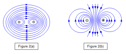
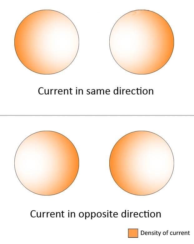
         2. Proximity Effect

            
         3. Corona

            \(\begin{array}{l c l} \text{Critical Disruptive Voltage} &:& \text{Corona is initiated} \\ & & V_c = E_c r \ln\left(\displaystyle\frac{d}{r}\right) = m_\circ g_\circ \delta r \ln\left( \displaystyle\frac{d}{r} \right) \\ & & E_c = E_\circ \delta m \left( 1 + \displaystyle\frac{K}{\sqrt{\delta r}} \right) \\ & & \delta = \displaystyle\frac{p}{p_\circ} \frac{T_\circ}{T} \\ \text{Visual Critical Voltage} &:& \text{Corona is visible} \\ & & V_v = m_v g_\circ \delta r \left( 1 + \displaystyle\frac{0.301}{\sqrt\delta r} \right) \ln\left( \displaystyle\frac{d}{r} \right) = \displaystyle\frac{m_v}{m_\circ} \left( 1 + \displaystyle\frac{0.301}{\sqrt{\delta r}} \right) V_c \\ & & \delta = \displaystyle\frac{3.92 b}{273 + t^\circ C} \\ \text{Power Loss due to corona} &:& \text{Peek's Formula: } P_{corona} = \displaystyle\frac{242.2}{\delta} (f + 25) \sqrt{\displaystyle\frac{r}{d}} (V - V_c)^2 \times 10^{-5} kW/km/Ph \\ & & \text{Peterson's Formula: } P_{corona} = \displaystyle\frac{2.1 f V^2 F}{\left( \log_{10}(d/r) \right)^2} \times 10^{-9} kW/km/Ph \\ \end{array}\)
         4. Radio Interferance

            \( \boxed{\begin{array}{c} \text{Unbalanced} \\ \text{Loading}\end{array}} \rightarrow \boxed{\begin{array}{c} \text{Unbalanced} \\ \text{Currents}\end{array}} \rightarrow \boxed{\begin{array}{c} \text{Incomplete} \\ \text{Field Cancellation}\end{array}} \rightarrow \boxed{\begin{array}{c} \text{Residual} \\ \text{Magnetic Field}\end{array}} \rightarrow \boxed{\begin{array}{c} \text{EMF} \\ \text{Induced}\end{array}} \rightarrow \boxed{\begin{array}{c} \text{Radio} \\ \text{Interference}\end{array}} \)
            .
            \( \boxed{\begin{array}{c} \text{Unsymmetrical} \\ \text{Spacing}\end{array}} \rightarrow \boxed{\begin{array}{c} \text{No} \\ \text{Transposition}\end{array}} \rightarrow \boxed{\begin{array}{c} \text{Unequal} \\ \text{Phase Inductances}\end{array}} \rightarrow \boxed{\begin{array}{c} \text{Incomplete} \\ \text{Field Cancellation}\end{array}} \rightarrow \boxed{\begin{array}{c} \text{Residual} \\ \text{Magnetic Field}\end{array}} \rightarrow \boxed{\begin{array}{c} \text{EMF} \\ \text{Induced}\end{array}} \rightarrow \boxed{\begin{array}{c} \text{Radio} \\ \text{Interference}\end{array}} \)
            .
            \( \boxed{\begin{array}{c} \text{High} \\ \text{Voltage} \end{array}} \rightarrow \boxed{\begin{array}{c} \text{Strong} \\ \text{Field} \end{array}} \rightarrow \boxed{\begin{array}{c} \text{Air} \\ \text{Ionization} \end{array}} \rightarrow \boxed{\begin{array}{c}\text{Current Pulse}\\\text{(at each peak of 50 Hz)}\end{array}}\rightarrow \boxed{\begin{array}{c}\text{100 bursts}\\\text{per second} \end{array}} \rightarrow \boxed{\begin{array}{c} \text{Electromagnetic Noise} \\ \text{(Broadband)} \end{array}}\rightarrow \boxed{\begin{array}{c} \text{EMF} \\ \text{Induced}\end{array}} \rightarrow \boxed{\begin{array}{c} \text{Radio} \\ \text{Interference}\end{array}} \)
            .
            \( \boxed{\begin{array}{c} \text{Loose} \\ \text{Bolts} \end{array}} \rightarrow \boxed{\begin{array}{c} \text{Potential} \\ \text{Difference} \end{array}} \rightarrow \boxed{\begin{array}{c} \text{Dielectric} \\ \text{Breakdown} \end{array}} \rightarrow \boxed{\begin{array}{c} \text{Impulse} \\ \text{Current} \end{array}} \rightarrow \boxed{\begin{array}{c} \text{Impulse} \\ \text{Radiowave} \end{array}} \rightarrow \boxed{\begin{array}{c} \text{EMF} \\ \text{Induced}\end{array}} \rightarrow \boxed{\begin{array}{c} \text{Radio} \\ \text{Interference}\end{array}} \)
         5. Ferranti Effect

            \(\begin{array}{l} |V_R| > |V_S| \\ 0 < \text{Short Line} < \text{Sending End C} < \text{T = } \pi < \text{Receiving End C} \end{array}\)
         6. Galloping

            \( \boxed{\begin{array}{c} \text{Irregular conductor shape} \\ \text{+} \\ \text{Moderate to high winds} \end{array}} \rightarrow \boxed{\begin{array}{c} \text{disrupted} \\ \text{smooth air flow} \\ \text{around the conductor} \end{array}} \rightarrow \boxed{\begin{array}{c} \text{aerodynamic lift & drag forces} \\ \text{+} \\ \text{elasticity & weight of the conductor} \end{array}} \rightarrow \boxed{\begin{array}{c} \text{twisting or torsional motion} \\ \text{+} \\ \text{vertical & horizontal movements} \end{array}} \rightarrow \boxed{\begin{array}{c} \text{oscillations with} \\ \text{high amplitude (more than sag),} \\ \text{low frequency (0.1 to 3 hz) motion} \end{array}} \)
            
         7. Aeolian Vibrations

            \( \boxed{\begin{array}{c} \text{bare conductor} \\ \text{+} \\ \text{smooth wind} \end{array}} \rightarrow \boxed{\begin{array}{c} \text{flow} \\ \text{separation} \end{array}} \rightarrow \boxed{\begin{array}{c} \text{vacuum} \\ \text{effect} \end{array}} \rightarrow \boxed{\begin{array}{c} \text{Vortex Street} \\ \boxed{\begin{array}{c c c} \boxed{\text{vortex growth on top}}&\rightarrow&\boxed{\text{vortex detach on top}}\\ \uparrow & & \downarrow \\ \boxed{\text{vortex growth on bottom}}&\leftarrow&\boxed{\text{vortex growth on bottom}}\\\end{array}}\end{array}} \rightarrow \boxed{\begin{array}{c} \text{creation of} \\ \text{alternating forces} \end{array}} \rightarrow \boxed{\begin{array}{c} \text{oscillations with} \\ \text{low amplitude (less than conductor dia),} \\ \text{high frequency (3 to 150 hz) motion} \end{array}} \)
            
      6. Performance Indices of Transmission Lines

         1. Voltage Regulation

            \(\begin{array}{l} VR = \displaystyle\frac{|\frac{V_S}{A}| - |V_R|}{|V_R|} \times 100\% \\ \end{array}\)
         2. Efficiency
      7. UG Cables

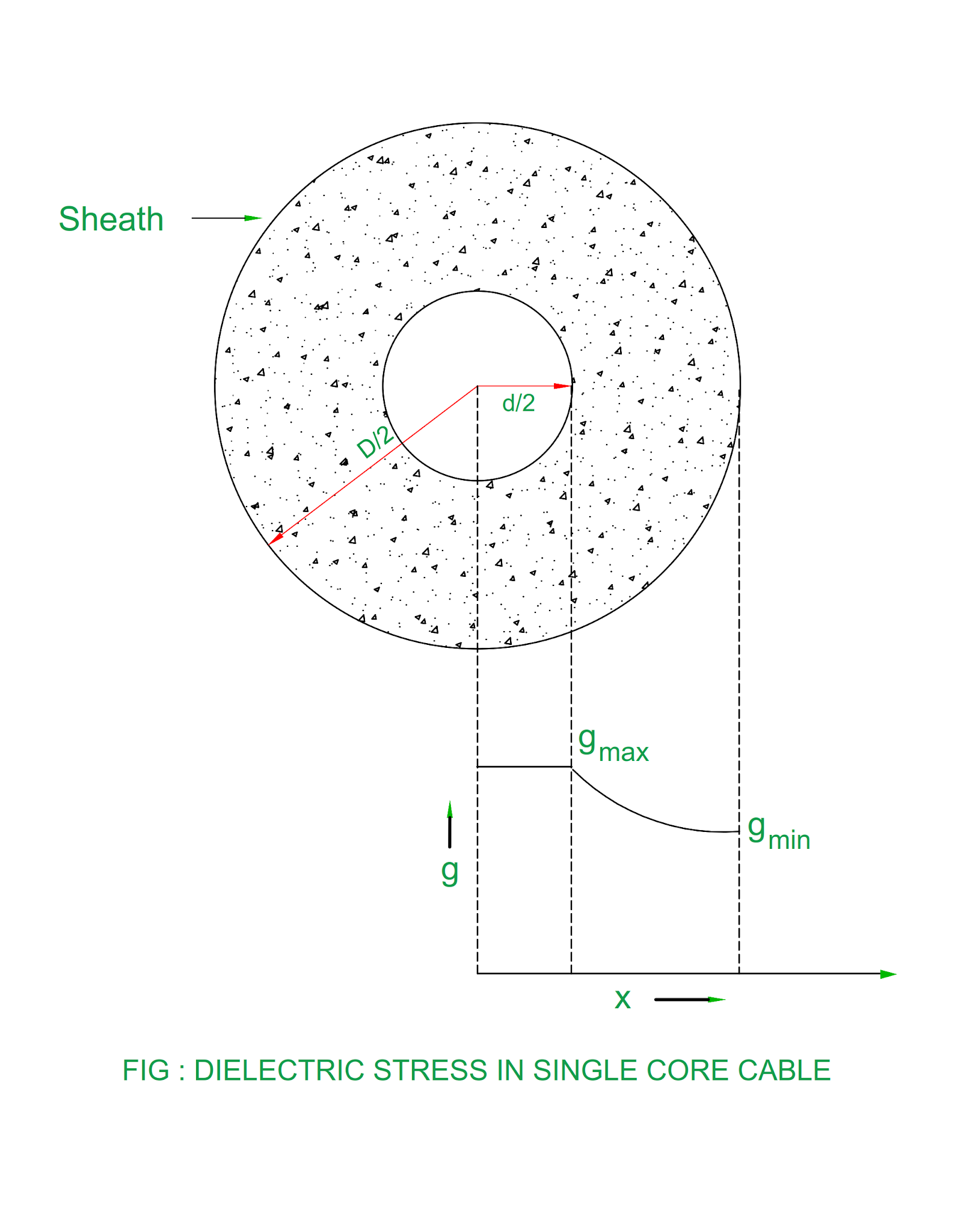
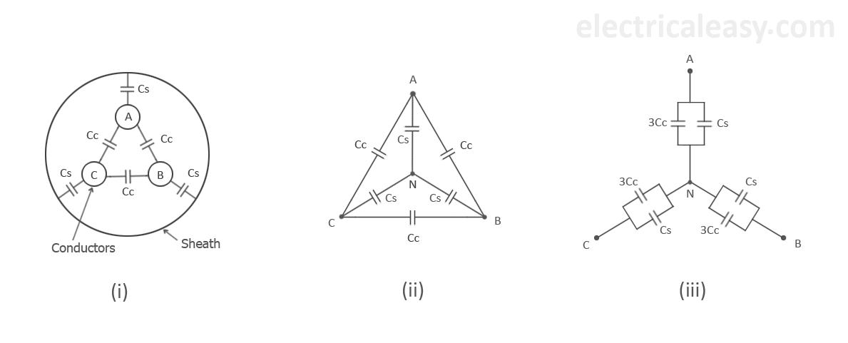
         \(\begin{array}{l c l} \text{Layers} &:& \text{Clever Ingineers Shield Before Armoring Serves} \\ \text{Insulation Resistance} &:& R_{ins} = \rho_{ins}\displaystyle\frac{\ln{R/r}}{2\pi{l}} \\ \text{Insulation Grading} &:& \text{To equalize the Electric stress} \\ & & \text{Quality insulator (high } E_{max}\epsilon_r \text{ near conductor} \\ \text{Cable Capacitance} &:& C_{\text{1 core}} = \displaystyle\frac{2\pi\epsilon}{\ln{(R/r)}} \\ & & C_{\text{3 core}} = C_{ph} = C_{cs} + 3C_{cc} \\ & & \text{2 cores shorted with sheath: } C_{1, cs} = C_{cs} + 2C_{cc} \\ & & \text{3 cores mutually shorted: } C_{2, cs} = 3C_{cs} \\ & & \Rightarrow C_{cs}=\displaystyle\frac{C_2}{3} ,\quad C_{cc}=\displaystyle\frac{C_1}{2} - \displaystyle\frac{C_2}{6} \\ & & \text{1 core shorted with sheath: } C_{3, cc} = C_{cc} + \displaystyle\frac{C_{cc} + C_{cs}}{2} = \displaystyle\frac{C_{ph}}{2} \Rightarrow C_{ph} = 2C_{3, cc} \\ \text{Dielectric Loss} &:& P_{loss, ph} = \omega C_{ph} V_{ph}^2 \tan\delta \\ \end{array}\)
         
      8. HVDC

         \(\begin{array}{l c l} \textbf{Monopolar Link} &:& \text{1 -ve conductor, +ve is grounded} \\ \textbf{Bipolar Link} &:& \text{2 conductors +ve and -ve, neutral is grounded} \\ \textbf{Homopolar Link} &:& \text{2 conductors -ve and +ve is grounded} \\ \end{array}\)
      9. Bus-Admittance [\(Y_{bus}\)] Matrix

         1. Current Equation: \([I_{bus}]=[Y_{bus}][V_{bus}]\)
         2. Voltage Equation: \([V_{bus}]=[Z_{bus}][I_{bus}] ,\quad [Z_{bus}]=[Y_{bus}]^{-1}\)
         3. [\(Y_{bus}\)] Building

            1. Diagonal or Driving Point Admittance: \(\sum{\text{Admittances Connected to the Respective Bus}} + \text{Admittance Connected between Respective Bus and Ground}\)
            2. Off Diagonal or Transfer Admittance: \(-\text{Admittance Connected between two Buses} \Rightarrow [Y_{bus}]\text{ is Symmetric}\)
            3. Sum of Each Row: \(\text{Admittance Connected between Respective Bus and Ground}\)
            4. Density of \([Y_{bus}]\): \(\displaystyle\frac{No. of Non-Zero Elements}{Total No. of Elements}\)
            5. Total No. of Elements: \(n^2 ,\quad \text{n = No. of Buses}\)
            6. No. of Non-Zero Elements: \(\text{Diagonal}+(2\times\text{No. of Transmission Lines})\)
            7. Sparsity of \([Y_{bus}]\): \(\displaystyle\frac{No. of Zero Elements}{Total No. of Elements} ,\quad \text{Sparsity of }[Y_{bus}] > \text{Density of }[Y_{bus}]\Rightarrow[Y_{bus}]\text{ is a Sparse Matrix}\)
      10. Bus-Impedance \([Z_{bus}]\) Matrix

          1. Bus Voltage: \([V_{bus}]=[Z_{bus}][I_{bus}] ,\quad [Z_{bus}]=[Y_{bus}]^{-1}\)
          2. Bus (Injected) Current: \([I_{bus}]=[Y_{bus}][V_{bus}]\)
          3. \([Z_{bus}]\text{ Elements}\)

             1. Diagonal Elements: Driving Point Thevenin Impedance
             2. Off Diagonal Elements: Transfer Impedance
          4. \([Z_{bus}]\text{ Building}\)

             1. Addition of New Bus to the existing \(k^{th}\) Bus through an Impedance, \(Z_b\)

                \(\begin{bmatrix}V_1\\\vdots\\V_k\\\vdots\\V_n\\V_p\end{bmatrix}=\begin{bmatrix} Z_{11}&\cdots& Z_{1k}&\cdots & Z_{1n}& Z_{1k}\\ \vdots&\vdots& \vdots&\vdots &\vdots &\vdots\\ Z_{k1}&\cdots& Z_{kk}&\cdots & Z_{kn}& Z_{kk}\\ \vdots&\vdots& \vdots&\vdots &\vdots &\vdots\\ Z_{n1}&\cdots& Z_{nk}&\cdots & Z_{nn}& Z_{nk}\\ Z_{k1}&\cdots& Z_{kk}&\cdots & Z_{kn}& Z_{kk}+Z_b\end{bmatrix} \begin{bmatrix}I_1\\\vdots\\I_k\\\vdots\\I_n\\I_p\end{bmatrix}\)
             2. Addition of New Bus, \(P^{th}\) or \((n+1)^{th}) Bus to a Reference Bus

                \(\begin{bmatrix}V_1\\\vdots\\V_k\\\vdots\\V_n\\V_p\end{bmatrix}=\begin{bmatrix} Z_{11}&\cdots& Z_{1k}&\cdots & Z_{1n}& Z_{1k}\\ \vdots&\vdots& \vdots&\vdots &\vdots &\vdots\\ Z_{k1}&\cdots& Z_{kk}&\cdots & Z_{kn}& Z_{kk}\\ \vdots&\vdots& \vdots&\vdots &\vdots &\vdots\\ Z_{n1}&\cdots& Z_{nk}&\cdots & Z_{nn}& Z_{nk}\\ Z_{k1}&\cdots& Z_{kk}&\cdots & Z_{kn}& Z_{kk}+Z_b\end{bmatrix} \begin{bmatrix}I_1\\\vdots\\I_k\\\vdots\\I_n\\I_p\end{bmatrix} ,\quad \text{Last Row, Last Column Elements = 0 Except }Z_{kk}+Z_b \to Z_p\)
                \(\begin{bmatrix}V_1\\\vdots\\V_n\\V_p\end{bmatrix}=\begin{bmatrix} Z_{11}&\cdots& Z_{1n}& 0\\\vdots&\vdots&\vdots&\vdots\\Z_{n1}&\cdots& Z_{nn}& 0\\0& 0& 0& Z_{p}\end{bmatrix} \begin{bmatrix}I_1\\\vdots\\I_n\\I_p\end{bmatrix}\)
             3. Addition of \(Z_p\) between an existing, \(k^{th}\) Bus and Reference\)

                \(\begin{bmatrix}V_1\\\vdots\\V_k\\\vdots\\V_n\\V_p\end{bmatrix}=\begin{bmatrix} Z_{11}&\cdots& Z_{1k}&\cdots & Z_{1n}& Z_{1k}\\ \vdots&\vdots& \vdots&\vdots &\vdots &\vdots\\ Z_{k1}&\cdots& Z_{kk}&\cdots & Z_{kn}& Z_{kk}\\ \vdots&\vdots& \vdots&\vdots &\vdots &\vdots\\ Z_{n1}&\cdots& Z_{nk}&\cdots & Z_{nn}& Z_{nk}\\ Z_{k1}&\cdots& Z_{kk}&\cdots & Z_{kn}& Z_{kk}+Z_b\end{bmatrix} \begin{bmatrix}I_1\\\vdots\\I_k\\\vdots\\I_n\\I_p\end{bmatrix} ,\quad V_p=0 ,\quad I_p=\begin{matrix}n\\\sum\\j=1\end{matrix}{c_jI_j}\) \([Z_{bus}]^{(new)}=[Z_{bus}]^{(old)}-\displaystyle\frac{XX^T}{Z_{pp}}, \quad Z_{pp}=Z_{kk}+Z_b ,\quad X=k^{th}\text{ column of the original matrix}\)
             4. Addition of \(Z_b\) between two existing, \(k^{th}\) and \(j^{th}\) Buses

                \(\begin{bmatrix}V_1\\\vdots\\V_k\\\vdots\\V_n\\V_p\end{bmatrix}=\begin{bmatrix} Z_{11}&\cdots& Z_{1k}&\cdots & Z_{1n}& Z_{1k}\\ \vdots&\vdots& \vdots&\vdots &\vdots &\vdots\\ Z_{k1}&\cdots& Z_{kk}&\cdots & Z_{kn}& Z_{kk}\\ \vdots&\vdots& \vdots&\vdots &\vdots &\vdots\\ Z_{n1}&\cdots& Z_{nk}&\cdots & Z_{nn}& Z_{nk}\\ Z_{k1}&\cdots& Z_{kk}&\cdots & Z_{kn}& Z_{kk}+Z_b\end{bmatrix} \begin{bmatrix}I_1\\\vdots\\I_k\\\vdots\\I_n\\I_b\end{bmatrix} ,\quad V_k-V_j=I_bZ_b ,\quad I_b=\begin{matrix}n\\\sum\\j=1\end{matrix}{c_jI_j}\) \([Z_{bus}]^{(new)}=[Z_{bus}]^{(old)}-\displaystyle\frac{XX^T}{Z_{pp}}, \quad Z_{pp}=Z_b+Z_{jj}+Z_{kk}-2Z_{jk} ,\quad X=k^{th}\text{ column }-j^{th}\text{ column of the original matrix}\)
             5. Removal of a Transmission Line Between two Buses

                \(\begin{bmatrix}V_1\\\vdots\\V_k\\\vdots\\V_n\\V_p\end{bmatrix}=\begin{bmatrix} Z_{11}&\cdots& Z_{1k}&\cdots & Z_{1n}& Z_{1k}\\ \vdots&\vdots& \vdots&\vdots &\vdots &\vdots\\ Z_{k1}&\cdots& Z_{kk}&\cdots & Z_{kn}& Z_{kk}\\ \vdots&\vdots& \vdots&\vdots &\vdots &\vdots\\ Z_{n1}&\cdots& Z_{nk}&\cdots & Z_{nn}& Z_{nk}\\ Z_{k1}&\cdots& Z_{kk}&\cdots & Z_{kn}& Z_{kk}+Z_b\end{bmatrix} \begin{bmatrix}I_1\\\vdots\\I_k\\\vdots\\I_n\\I_b\end{bmatrix} ,\quad \text{Add an Impedance of -Z between those two buses}\)
3. Load Flow Analysis

   1. Static Power Transfer Equation

      \(\begin{array}{l} \bar{S}_S = \bar V_S \bar I_S^{*} = |V_S|\angle{\delta} \left[\displaystyle\frac{|D|}{|B|}|V_S|\angle{\beta-\Delta-\delta}-\displaystyle\frac{|V_R|}{|B|}\angle{\beta}\right] = \displaystyle\frac{|D|}{|B|}|V_S|^2\angle{\beta-\Delta} - \displaystyle\frac{|V_S| |V_R|}{|B|}\angle{\beta+\delta} \approx \left[\displaystyle\frac{1}{X}|V_S|^2\angle{90^\circ}\right] - \left[\displaystyle\frac{|V_S| |V_R|}{X}\angle{(90^\circ-\delta)}\right] \\ \bar{S}_R = \bar V_R \bar I_R^{*} = |V_R|\angle{0} \left[\displaystyle\frac{|V_S|}{|B|}\angle{\beta-\delta} - \displaystyle\frac{|A|}{|B|}|V_R|\angle{\beta-\alpha}\right] = \displaystyle\frac{|V_S| |V_R|}{|B|}\angle{\beta-\delta} - \displaystyle\frac{|A|}{|B|}|V_R|^2\angle{\beta-\alpha} \approx \left[\displaystyle\frac{|V_S| |V_R|}{X}\angle{(90^\circ-\delta)}\right] - \left[\displaystyle\frac{1}{X}|V_R|^2\angle{90^\circ}\right] \\ \end{array}\)
      Real Power Flows from Higher Load Angle to Lower Load Angle
      Reactive Power Flows from Higher Voltage to Lower Voltage
      \(\begin{array}{|c|c|c|}\hline \textbf{Sending End Reactive Power} & \textbf{Receiving End Reactive Power} & \textbf{Direction of Reactive Power} \\\hline Q_S > 0 \Rightarrow \text{Over Excited} & Q_R > 0 \Rightarrow \text{Inductive Load} & \text{Source gives to Line, Line gives to Load}\\\hline Q_S > 0 \Rightarrow \text{Over Excited} & Q_R < 0 \Rightarrow \text{Capacitive Load} & \text{Line absorbs from both source and load}\\\hline Q_S < 0 \Rightarrow \text{Under Excited} & Q_R > 0 \Rightarrow \text{Inductive Load} & \text{Line gives to both source and load}\\\hline Q_S < 0 \Rightarrow \text{Under Excited} & Q_R < 0 \Rightarrow \text{Capacitive Load} & \text{Load gives to Line, Line gives to Source}\\\hline \end{array}\)
   2. Bus Classification

      \(\begin{array}{l c l} \text{Generator Bus}&:&\text{PV-Bus}\\ & & Q_{gi}< Q_{gi(min)}\Rightarrow\text{PV-Bus becomes PQ-Bus}\\ & & Q_{gi}> Q_{gi(max)}\Rightarrow\text{PV-Bus becomes PQ-Bus}\\ \text{Load Bus}&:&\text{PQ-Bus}\\ & & V_{i}< V_{i(min)}\Rightarrow\text{PQ-Bus becomes PV-Bus}\\ & & V_{i}> V_{i(max)}\Rightarrow\text{PQ-Bus becomes PV-Bus}\\ \text{Voltage Controlled Bus}&:&\text{PV-Bus with no generator but with variable reactive power compensators}\\ & & \text{Buses with fixed shunt-L or fixed shunt-C are considered PQ buses}\\ \text{Reference Bus}&:&\text{Swing or Slack (Responsible) Bus: }V\delta\text{-Bus}\\ & & \text{If V is More (No Change from}\E_g\text{, No Droop generator) this bus belivers Q}\\ & & \text{If }\delta\text{ is More (Highest Capacity of all the other generators in the system) this bus belivers P}\\ \end{array}\)
   3. Load Flow Solution

      \(\begin{array}{l c l} \text{Basic Load Flow Equation}&:& S_i=S_{gi}-S_{di}=V_iI_i^{*}=P_i+jQ_i\\ & & S_i^{*}=V_i^{*}I_i=P_i-jQ_i\Rightarrow I_{i}=\displaystyle\frac{P_i-jQ_i}{V_i^{*}}\\ & & I_i=\begin{matrix}n\\\sum\\k=1\end{matrix}{Y_{ik}V_k} =Y_{ii}V_i+\begin{matrix}n\\\sum\\k=1\\k\neq i\end{matrix}{Y_{ik}V_k}\\ & & \Rightarrow V_i=\displaystyle\frac{1}{Y_{ii}}\left[\displaystyle\frac{P_i-jQ_i}{V_i^{*}} -\begin{matrix}n\\\sum\\k=1\\k\neq i\end{matrix}{Y_{ik}V_k}\right]\\ \text{Gauss Method}&:& V_i^{(m+1)}=\displaystyle\frac{1}{Y_{ii}}\left[\displaystyle\frac{P_i-jQ_i}{\left[V_i^{(m)}\right]^{*}} -\begin{matrix}n\\\sum\\k=1\\k\neq i\end{matrix}{Y_{ik}V_k^{(m)}}\right]\\ \text{Gauss-Seidel Method}&:& V_{i, GS}^{(m+1)}=\displaystyle\frac{1}{Y_{ii}}\left[\displaystyle\frac{P_i-jQ_i}{\left[V_i^{(m)}\right]^{*}} -\begin{matrix}i-1\\\sum\\k=1\end{matrix}{Y_{ik}V_k^{(m+1)}} -\begin{matrix}n\\\sum\\k=i+1\end{matrix}{Y_{ik}V_k^{(m)}}\right]\\ & &\text{Acceleration Factor, }\alpha=\text{1.3 to 1.6}\Rightarrow V_{i, acc}^{(m+1)}=V_i^{(m)}+\alpha\left(V_{i, GS}^{(m+1)}-V_i^{(m)}\right)\\ & &\text{Intermediate voltage, }V_{i, GS}^{(m+1)}\text{ is calculated using Gauss-Seidel formula and the}\\ & & \text{acceleration formula is applied on the intermediate voltage to get a final improved voltage, }V_{i, acc}^{(m+1)}\\ & & \text{and then immediately this final value is used to solve for the very next bus within the same iteration}\\ & & \text{to achieve faster overall convergence}\\ \text{Newton-Raphson Method}&:& \text{Missmatch Vector}=\text{Jacobian}\times\text{Correction Vector}\Rightarrow \begin{bmatrix}\Delta P\\\Delta Q\end{bmatrix}_{(2PQ+PV)\times(1)}= \begin{bmatrix}\displaystyle\frac{\partial P}{\partial\delta}&\displaystyle\frac{\partial P}{\partial|V|}\\ \displaystyle\frac{\partial Q}{\partial\delta}&\displaystyle\frac{\partial Q}{\partial|V|}\end{bmatrix}_{(2PQ+PV)\times(2PQ+PV)} \begin{bmatrix}\Delta\delta\\\Delta|V|\end{bmatrix}_{(2PQ+PV)\times(1)}\\ & & \Rightarrow \begin{bmatrix}\Delta P\\\Delta Q\end{bmatrix}_{(2PQ+PV)\times(1)}= \begin{bmatrix}[J_1]_{(PQ+PV)\times(PQ+PV)}&[J_2]_{(PQ+PV)\times(PQ)}\\ [J_3]_{(PQ)\times(PQ+PV)}&[J_4]_{(PQ)\times(PQ)}\end{bmatrix}_{(2PQ+PV)\times(2PQ+PV)} \begin{bmatrix}\Delta\delta\\\Delta|V|\end{bmatrix}_{(2PQ+PV)\times(1)}\\ & & \Rightarrow[J]=\begin{bmatrix}(\text{P is known on which buses})\times(\delta\text{ is unknown on which buses})& (\text{P is known on which buses})\times(|V|\text{ is unknown on which buses})\\ (\text{Q is known on which buses})\times(\delta\text{ is unknown on which buses})& (\text{Q is known on which buses})\times(|V|\text{ is unknown on which buses}) \end{bmatrix}\\ & & \Rightarrow \begin{bmatrix}\Delta\delta\\\Delta|V|\end{bmatrix}_{(2PQ+PV)\times(1)}= \begin{bmatrix}\displaystyle\frac{\partial P}{\partial\delta}&\displaystyle\frac{\partial P}{\partial|V|}\\ \displaystyle\frac{\partial Q}{\partial\delta}&\displaystyle\frac{\partial Q}{\partial|V|}\end{bmatrix}^{-1} \begin{bmatrix}\Delta P\\\Delta Q\end{bmatrix}_{(2PQ+PV)\times(1)}\\ \text{Fast Decoupled Load Flow}&:&\displaystyle\frac{\partial P}{\partial|V|}=0 ,\quad \displaystyle\frac{\partial Q}{\partial\delta}=0\\ & & \Rightarrow \begin{bmatrix}\Delta\delta\\\Delta|V|\end{bmatrix}_{(2PQ+PV)\times(1)}= \begin{bmatrix}\displaystyle\frac{\partial P}{\partial\delta}& 0\\ 0 &\displaystyle\frac{\partial Q}{\partial|V|}\end{bmatrix}^{-1} \begin{bmatrix}\Delta P\\\Delta Q\end{bmatrix}_{(2PQ+PV)\times(1)}\\ \end{array}\)
      \(\begin{array}{|l|l|l|l|}\hline \textbf{Criteria} & \textbf{GS} & \textbf{N-R} & \textbf{FD} \\\hline \text{Calculation} & \text{Easy} & \text{Highest} & \text{Moderate} \\\hline \text{Number of iteration} & \text{Large} & \text{Moderate} & \text{Least} \\\hline \text{Time taken for 1 iteration} & \text{Least} & \text{Highest} & \text{Moderate} \\\hline \text{Convergence} & \text{Linear} & \text{Quadratic} & \text{Geometric} \\\hline \text{Accuracy} & \text{Good} & \text{Best} & \text{Good} \\\hline \end{array}\)
4. Fault Analysis

   1. Per Unit System

      1. Given Bases: \(V_{l.b} ,\quad S_{3\phi.{b}}\)
      2. Derived Bases: \(I_{l.b} = \displaystyle\frac{S_{3\phi.{b}}}{\sqrt{3}V_{l.b}} ,\quad Z_b = \displaystyle\frac{V_{ph.b}}{I_{ph.b}}\)
      3. PU quantity: \(\text{per unit value} = \displaystyle\frac{\text{actual value}}{\text{base value}}\)
      4. Change of Base: \(\text{new per unit value} = \displaystyle\frac{\text{old per unit value} \times \text{old base}}{\text{new base}}\)
   2. Types of Faults

      1. Open Circuit Faults

         1. One Line Open

            1. Near The Generator
            2. At a Far End on the Line
         2. Two Lines Open

            1. Near The Generator
            2. At a Far End on the Line
         3. All Three Lines Open

            1. Near The Generator
            2. At a Far End on the Line
      2. Short Circuit Faults

         1. Symmetrical Short Circuit Faults

            1. LLL Faults

               1. Near The Generator
               2. At a Far End on the Line
            2. LLLG Faults

               1. Near The Generator
               2. At a Far End on the Line
         2. Unsymmetrical Short Circuit Faults

            1. LG Faults

               1. Near The Generator
               2. At a Far End on the Line
            2. LL Faults

               1. Near The Generator
               2. At a Far End on the Line
            3. LLG Faults

               1. Near The Generator
               2. At a Far End on the Line
   3. Symmetrical Components

      1. Sequence Components

         \(\begin{array}{l c l} \text{Idea} &:& \text{Unbalanced system = (+ve sequence + -ve sequence + 0 sequence) components}\\ && V_a=V_{a1}+V_{a2}+V_{a0}\\ && V_b=V_{b1}+V_{b2}+V_{b0}=\alpha^2V_{a1}+\alpha V_{a2}+V_{a0}\\ && V_c=V_{c1}+V_{c2}+V_{c0}=\alpha V_{a1}+\alpha^2V_{a2}+V_{a0}\\ && \begin{bmatrix}V_a\\V_b\\V_c\end{bmatrix} = \begin{bmatrix}1& 1& 1\\\alpha^2&\alpha& 1\\\alpha&\alpha^2& 1\end{bmatrix} \begin{bmatrix}V_{a1}\\V_{a2}\\V_{a0}\end{bmatrix} \Rightarrow \begin{bmatrix}V_{a1}\\V_{a2}\\V_{a0}\end{bmatrix} = \frac{1}{3} \begin{bmatrix}1&\alpha&\alpha^2\\1&\alpha^2&\alpha\\1& 1& 1\end{bmatrix} \begin{bmatrix}V_a\\V_b\\V_c\end{bmatrix}\\ && \begin{bmatrix}V_a\\V_b\\V_c\end{bmatrix} = \begin{bmatrix}1& 1& 1\\1&\alpha^2&\alpha\\1&\alpha&\alpha^2\end{bmatrix} \begin{bmatrix}V_{a0}\\V_{a1}\\V_{a2}\end{bmatrix} \Rightarrow \begin{bmatrix}V_{a0}\\V_{a1}\\V_{a2}\end{bmatrix} = \frac{1}{3} \begin{bmatrix}1& 1& 1\\1&\alpha&\alpha^2\\1&\alpha^2&\alpha\end{bmatrix} \begin{bmatrix}V_a\\V_b\\V_c\end{bmatrix}\\ && S = \begin{bmatrix}V_a& V_b& V_c\end{bmatrix} \begin{bmatrix}I_a\\I_b\\I_c\end{bmatrix}^{*} = \begin{bmatrix}V^{abc}\end{bmatrix}^T \begin{bmatrix}I^{abc}\end{bmatrix}^{*} = 3 \begin{bmatrix}V^{012}\end{bmatrix}^T \begin{bmatrix}I^{012}\end{bmatrix}^{*}\\ && \text{Neutral Current, }I_n=I_a+I_b+I_c=3I_{a0}\\ \end{array}\)
      2. Sequence Networks

         1. Y-Load: \(Z_1=Z_2=Z_{load} ,\quad Z_0=Z_{load}+3Z_{grounding}\)
         2. \(\Delta\)-Load: \(Z_1=Z_2=\frac{Z_{load}}{3} ,\quad Z_0=\infty ,\quad I_0 \text{ in loop}\)
         3. Y-Alternator: \(Z_1=\begin{cases}jX_d^{"} & \text{(sub-transient)}\\ jX_d^{'} & \text{(transient)}\\ jX_d & \text{(steady-state)}\end{cases} ,\quad Z_2=j\displaystyle\frac{X_d^{"}+X_q^{"}}{2} ,\quad Z_0=Z_{g0}+3Z_{grounding}\)
         4. \(\Delta\)-Alternator: \(Z_1=\begin{cases}jX_d^{"} \text{ (sub-transient)}\\ jX_d^{'} \text{ (transient)}\\ jX_d \text{ (steady-state)}\end{cases} ,\quad Z_2=j\displaystyle\frac{X_d^{"}+X_q^{"}}{2} ,\quad Z_0=\infty ,\quad I_0 \text{ in loop}\)
         5. Transformer: \(Z_1=Z_2=jX_l ,\quad Z_0=\text{depends on star/ delta on primary and secondary}\)
         6. Transmission Line: \(Z_1=Z_2=Z_{line} ,\quad Z_0\approx3Z_1=3Z_2\)
   4. Transients

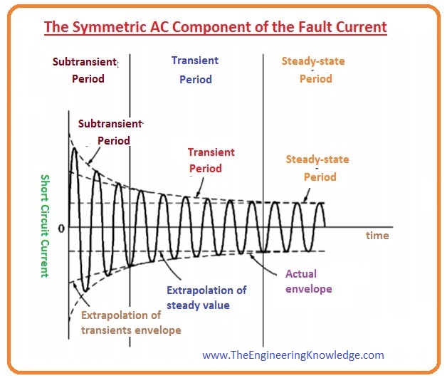
      \(\begin{array}{l c l} \text{Transient Current Equation} &:& i = \displaystyle\frac{V_m}{|Z|}\sin{(\theta-\alpha)}e^{-t/\tau} + \displaystyle\frac{V_m}{|Z|} \sin{[\omega t- (\theta - \alpha)]} ,\quad \phi = \tan^{-1}\frac{\omega L}{R}\\ && \text{first 3 cycles are sub-transient period}\\ && \text{sub-transient period: Rapid Decay: damper winding action}\\ && \text{next 30 cycles are transient period}\\ && \text{transient period: Slower Decay: Main field action: CB Operation Period}\\ && \text{Sub-transient reactance, }X_d^{"} < \text{transient reactance, }X_d^{'} < \text{steady state, }X_d\\ \text{Asymmetrical RMS } I_{fault}&:& I_{asy, rms} = \sqrt{{DC}^2+{AC}^2}=\displaystyle\frac{V_m}{\sqrt{2}|Z|}\\ && \text{asymmetrical: decaying dc + decaying ac}\\ && \text{decaying ac: due to varying reactance}\\ \text{Maximum Momentary Current} &:& I_{mm} \approx 2.55 \times I_{asy, rms}\\ \end{array}\)
      
      
   5. Fault Reactance

      \(\begin{array}{l c l} \text{Before the Fault} &:& \text{Steady State Reactance, } X_d\\ \text{During the Fault} &:& \text{Sub-Transient Reactance, } X_d^{"}\\ \text{After the Fault} &:& \text{Transient Reactance, } X_d^{'}\\ \text{Final Settling Point} &:& \text{Steady State Reactance, } X_d\\ \text{Order of Magnitude} &:& X_d^{"} < X_d^{"} < X_d\\ \end{array}\)
      
   6. Fault Classification

      1. Series (Open Circuit) Faults

         1. One Phase Open
         2. Two Phases Open
         3. All Three Phases Open
      2. Shunt (Short Circuit) Faults

         1. Symmetrical Short Circuit Faults

            1. LLLG: Most Severe on Transmission Lines
            2. LLL
         2. Unsymmetrical Short Circuit Faults

            1. LLG
            2. LL
            3. LG: Most Severe near alternator, Most Frequent on transmission lines
   7. Symmetrical Fault Analysis

      1. LLL Fault

         \(\begin{array}{l c l} \text{Fault Current} &:& I_f=I_{a1}=\displaystyle\frac{E}{Z_{+ve}+Z_{fault}}\\ \text{Short Circuit MVA} &:& \text{SC-MVA} = \text{SC-MVA}_{\text{pu}} \times S_{base} \Rightarrow \text{SC-MVA}_{\text{pu}} = I_{a1, pu}^{*}=\displaystyle\frac{1}{Z_{+ve}+Z_{fault}}\\ \end{array}\)
      2. LLLG Fault

         \(\begin{array}{l c l} \text{Fault Current} &:& I_f=I_{a1}\displaystyle\frac{E}{Z_{+ve}}\\ \text{Short Circuit MVA} &:& \text{SC-MVA} = \text{SC-MVA}_{\text{pu}} \times S_{base} \Rightarrow \text{SC-MVA}_{\text{pu}} = I_{a1, pu}^{*}=\displaystyle\frac{1}{Z_{+ve}}\\ \end{array}\)
   8. Unsymmetrical Fault Analysis

      1. LG Fault

         \(\begin{array}{l c l} \text{Fault Current} &:& I_{a1}=I_{a2}=I_{a0}=\displaystyle\frac{I_a}{3} \Rightarrow I_f = 3I_{a1} = \displaystyle\frac{V_a}{3Z_{fault}} = \displaystyle\frac{E_a}{Z_1+Z_2+Z_0+3Z_n+3Z_{fault}}\\ \text{Short Circuit MVA} &:& \text{SC-MVA} = \text{SC-MVA}_{\text{pu}} \times S_{\text{base}} ,\quad \text{SC-MVA}_{\text{pu}} = I_{a1, pu}\\ \end{array}\)
      2. LL Fault

         \(\begin{array}{l c l} \text{Fault Current} &:& I_{a1}=-I_{a2}=j\displaystyle\frac{I_b}{\sqrt{3}} ,\quad I_a0=0 ,\quad I_f=I_b=-j\sqrt{3}I_{a1} ,\quad I_{a1}=\displaystyle\frac{E_a}{Z_1+Z_2+Z_f} \Rightarrow I_{a1, pu}=\displaystyle\frac{1}{Z_1+Z_2+Z_f}\\ \text{Short Circuit MVA} &:& \text{SC-MVA} = \text{SC-MVA}_{\text{pu}} \times S_{\text{base}} ,\quad \text{SC-MVA}_{\text{pu}} = I_{a1, pu}\\ \end{array}\)
      3. LLG Fault

         \(\begin{array}{l c l} \text{Fault Current} &:& I_f=I_b+I_c=3I_{a0} ,\quad I_{a0}=\frac{V_{a0}-V_{a1}}{3Z_{fault}}=\frac{V_{a0}-V_{a2}}{3Z_{fault}} ,\quad I_{a1}=\displaystyle\frac{E_a}{Z_1+ [Z_2\parallel(Z_0+3Z_n+3Z_f)]} I_{a1, pu}=\displaystyle\frac{1}{Z_1+ [Z_2\parallel(Z_0+3Z_n+3Z_f)]} I_{a0}=-\displaystyle\frac{I_{a1}Z_2}{Z_2+Z_0+3Z_n+3Z_f}\\ \text{Short Circuit MVA} &:& \text{SC-MVA} = \text{SC-MVA}_{\text{pu}} \times S_{\text{base}} ,\quad \text{SC-MVA}_{\text{pu}} = I_{a1, pu}\\ \end{array}\)
   9. Fault Analysis With \([Z_{bus}]\) Matrix

      \(\begin{array}{l c l} \text{Fault Current}&:&\displaystyle\frac{V_{prefault}}{Z_{+ve}+Z_{fault}}=\displaystyle\frac{V_{pf, i}}{Z_{ii}+Z_{fault}} ,\quad Z_{ii}=Z_{th} \text{ of }i^{th}\text{ bus}\\ \text{Fault at }k^{th}\text{ bus on No-Load}&:& \Delta V_k=0 ,\quad \Delta I_k=-I_{fault} ,\quad [V]=[Z][I]\Rightarrow[\Delta V]=[Z][\Delta I] \\ & & \Delta V_k=-I_{fault}Z_{kk} ,\quad I_{fault}=\displaystyle\frac{V_k}{Z_{kk}+Z_{fault}}\approx\displaystyle\frac{V_k}{Z_{kk}}\\ & & \text{Change in Voltage of }j^{th}\text{ bus: }\Delta V_j=Z_{jk}(-I_{fault})=-Z_{jk}\displaystyle\frac{V_k}{Z_{kk}} \Rightarrow V_j^{(new)}=V_j^{(old)}+\Delta V_j=V_j-\displaystyle\frac{Z_{jk}}{Z_{kk}}V_k\\ & & \text{Fault Current supplied by the generator at }j^{th}\text{ bus: }I_j=\displaystyle\frac{E_j-V_j^{(new)}}{jX_d^{"}} =\displaystyle\frac{V_j^{(old)}-V_j^{(new)}}{jX_d^{"}}=\displaystyle\frac{Z_{jk}}{Z_{kk}}\times\displaystyle\frac{V_k}{jX_D^{"}}\\ \end{array}\)
5. Stability Analysis

   1. Voltage Stability (\( \pm 5\% \))

      1. Generator Side Voltage Control - Automatic Voltage Regulator
      2. Load Side Voltage Control

         1. Shunt Compensation - Q control

            1. Shunt Capacitor - To Compensate for Lagging Loads

               \(\begin{array}{l} |V_R| = |V_S| - \displaystyle\frac{X}{|V_S|}Q_S \\ \textbf{Before: } |V_{R1}| = |V_S| - \displaystyle\frac{X}{|V_S|}Q_S = |V_S| - \displaystyle\frac{X}{|V_S|}Q_{load} \\ \textbf{After: } Q_S=Q_{load}-Q_{Sh}\Rightarrow|V_{R2}|=|V_S|-\displaystyle\frac{X}{|V_S|}Q_{load}+\displaystyle\frac{X}{|V_S|}Q_{Sh}\\ \Delta{|V_R|} = |V_{R2}| - |V_{R1}| = \displaystyle\frac{X}{|V_S|}Q_{Sh} \text{ from here Q_{Sh} needed for desired |V_R| is calculated} \\ \hline \textbf{Before: } S_1 = P_L + jQ_L \Rightarrow \phi_1 = \tan^{-1}\displaystyle\frac{Q_L}{P_L} \\ \textbf{After: } S_2 = P_L + j(Q_L - Q_{Sh}) \Rightarrow \phi_2 = \tan^{-1}\displaystyle\frac{Q_L-Q_{Sh}}{P_L} \Rightarrow \text{ pf improved}\\ \end{array}\)
            2. Shunt Reactor - To Compensate for Ferranti Effect

               \(\begin{array}{l} |V_R| = |V_S| - \displaystyle\frac{X}{|V_S|}Q_S \\ \textbf{Before: } |V_{R1}| = |V_S| - \displaystyle\frac{X}{|V_S|}Q_S = |V_S| + \displaystyle\frac{X}{|V_S|}Q_{load} \\ \textbf{After: } Q_S=Q_{Sh}-Q_{load}\Rightarrow|V_{R2}|=|V_S|+\displaystyle\frac{X}{|V_S|}Q_{load}-\displaystyle\frac{X}{|V_S|}Q_{Sh}\\ \Delta{|V_R|} = |V_{R1}| - |V_{R2}| = \displaystyle\frac{X}{|V_S|}Q_{Sh}\text{ from here }Q_{Sh}\text{ needed for desired |V_R| is calculated}\\ \textbf{Alternately: } X_{L(Sh)} = \displaystyle\frac{|B|}{1 - |A|} \\ \end{array}\)
         2. Series Compensation - X control

            1. Series Capacitor - To Increase Stability

               \(\begin{array}{l} \textbf{Before: } |V_S| - |V_{R1}| = IR\cos\phi_R + IX\sin\phi_R \\ \textbf{After: } |V_S| - |V_{R2}| = IR\cos\phi_R + I(X-X_C)\sin\phi_R \\ \Rightarrow |V_{R2}| - |V_{R1}| = IX_C\sin\phi_R \text{ by controlling } X_C, \Delta{V_R} \text{ can be controlled} \\ \hline \textbf{Before: } P_{max1} = \displaystyle\frac{|V_S||V_R|}{X} \\ \textbf{After: } P_{max2} = \displaystyle\frac{|V_S||V_R|}{X-X_C} \\ \Rightarrow \text{ by controlling } X_C, P_{max} \text{ can be controlled} \Rightarrow \text{Stability limit is increased} \\ \hline \textbf{Before: } I_{fault1} = \displaystyle\frac{|V_S|}{X} \\ \textbf{After: } I_{fault2} = \displaystyle\frac{|V_S|}{X-X_C} \\ \Rightarrow \text{ by controlling } X_C, V_R \text{ and } P_{max} \text{ are improved but the fault currents become detrimental}\\ \hline \text{LC oscillator (less than synchronous frequency) due to compensating series capacitor + turbine system natural frequency} \\ \Rightarrow \text{Sub-Synchronous Resonance} \Rightarrow \text{Transient Torques, Torsional Interactions and Induction Generator Effect} \\ \Rightarrow \text{Shaft Damage due to Fatigue and Equipment Damage} \\ \end{array}\)
            2. Series Reactor - To Control the Real Power Flow in the Parallel Lines Connected to the Same Bus Bar
         3. Dynamic Voltage Control - Using a Synchronous Condenser or a Synchronous Phase Modifier

            \(\begin{array}{|c|c|}\hline \textbf{Excitation} & \textbf{Reactive Power} \\\hline \text{Under Excited} & \text{Q is absorbed by the synchronous motor} \\\hline \text{Critically Excited} & \text{Q is neither absorbed nor delivered by the synchronous motor} \\\hline \text{Over Excited} & \text{Q is delivered by the synchronous motor} \\\hline \end{array}\)
         4. FACTS devices

            \(\begin{array}{l c l} \text{Sh-Static VAR Compensator}&:&\text{Thyristor Controlled Reactors:continuous}\\ &&\text{Thyristor Switched Reactors:stepped} \\ &&\text{Thyristor Switched Capacitors:stepped} \\ \text{Series compensators} &&\text{Thyristor Controlled Series Capacitor} \\ \text{Voltage Source Converters}&:&\text{Sh-STATCOM: Static Sync' Compensator}\\ &&\text{Se-SSSC: Static Sync' Series Compensator}\\ \text{Hybrid Converters}&:&\text{UPFC: Unified Power Flow Controller (Se+Sh)}\\ &&\text{IPFC: Interline Power Flow Controller (Se+Se)} \\ \end{array}\)
   2. Frequency Stability (\( \pm 2\% \))

      1. Primary Control - Speed Governor on Generator Side
      2. Secondary Control

         1. Flat Frequency Control - Excess Load is handled by 0 droop Generators
         2. Parallel Frequency Control - Excess Load is distributed between parallelly operating generators
         3. Flat Tie-Line Control - Tie-Line Power is Maintained Constant

            1. Area Frequency Response Characteristics

               \(\begin{array}{l} \Delta{f} \propto \Delta{P} \Rightarrow \Delta{f} = \displaystyle\frac{R}{1 + RB} \Delta{P} \\ R = -\displaystyle\frac{\partial{f}}{\partial{P_G}} ,\quad B = \displaystyle\frac{\partial{P_D}}{\partial{f}}\\ \end{array}\)
            2. Area Control Error

               \(\begin{array}{l} \text{ACE} = P_{\text{actual}}-P_{\text{scheduled}} = \Delta{P_{tie}} + B\Delta{f} \end{array}\)
   3. Power Angle Stability (\( 20^\circ \text{ to } 30^\circ\))

      1. Swing Equation

         \(\begin{array}{l c l} \text{Kinetic Energy, Mechanical} &:& K.E. = \displaystyle\frac{1}{2}Mv^2 \to \displaystyle\frac{1}{2}J\omega_{sm}^2\\ \text{Kinetic Energy, Electrical} &:& \theta_{e}=\displaystyle\frac{P}{2}\theta_{m} \Rightarrow \theta_m=\displaystyle\frac{2}{P}\theta_e \Rightarrow \displaystyle\frac{d\theta_m}{dt}=\displaystyle\frac{2}{P}\displaystyle\frac{d\theta_e}{dt} \Rightarrow \omega_{sm}=\displaystyle\frac{2}{P}\omega_s\\ & & K.E.=\displaystyle\frac{1}{2}J\omega_{sm}^2 =\displaystyle\frac{1}{2}M\omega_s ,\quad M=\displaystyle\frac{J\omega_s}{(P/2)^2} =\displaystyle\frac{K.E.}{(\omega_s/2)}MJ-s/^c(elec)\\ & & K.E.=S_{base}H=GH ,\quad H=\displaystyle\frac{K.E.}{G}MJ/MVA \Rightarrow M=\displaystyle\frac{GH}{\pi f}MJ-s/^c(elec)\\ \text{Swing Equation, Mechanical} &:& \tau_{net}=\tau_{shaft}-\tau_{electromagnetic} \Rightarrow J\displaystyle\frac{d^2\theta_m}{dt^2}=\tau_{shaft}-\tau_{electromagnetic}\\ \text{Swing Equation, Electrical} &:& J\frac{d^2\theta_m}{dt^2}=\tau_{sh}-\tau_{em} \Rightarrow M\displaystyle\frac{d^2\theta_e}{dt^2}=P_s-P_e\\ & &\theta_{e}=\omega_st+\delta\Rightarrow\displaystyle\frac{d\theta_e}{dt}=\omega_s+\displaystyle\frac{d\delta}{dt}\Rightarrow \omega=\omega_s+\displaystyle\frac{d\delta}{dt}\\ & & \displaystyle\frac{d\theta_e}{dt}=\omega_s+\displaystyle\frac{d\delta}{dt}\Rightarrow \displaystyle\frac{d^2\theta_e}{dt^2}=\displaystyle\frac{d^\delta}{dt^2}\Rightarrow M\displaystyle\frac{d^2\theta_e}{dt^2}=P_s-P_e\to M\displaystyle\frac{d^2\delta}{dt^2}=P_s-P_e\\ \text{Multi-Machine Systems} &:& \text{Coherent Swing: }\delta_1=\delta_2=\cdots=\delta_i \Rightarrow M=\sum{M_i} ,\quad P_s=\sum{P_{si}},\quad P_e=\sum{P_{ei}}\\ & &\text{Incoherent Swing: }\delta_1\neq\delta_2 \Rightarrow M^{-1}=M_1^{-1}+M_2^{-1}\\ \end{array}\)
      2. Steady State Stability

         \(\begin{array}{l c l} \text{Small Change in Load Angle} &:& \delta_{new}=\delta_{old}+\Delta\delta\\ & & P_e=P_{max}\sin\delta\Rightarrow P_{e, new}=P_{max}\sin(\delta_{old}+\Delta\delta) \Rightarrow P_{e, new}=P_{e, old}+P_{max}\cos\delta_{old}\Delta\delta\\ & & M\displaystyle\frac{d^2\delta}{dt^2}=P_s-P_e \Rightarrow M\displaystyle\frac{d^2\delta_{new}}{dt^2}=P_s-P_{e,new}\\ & & \Rightarrow M\displaystyle\frac{d^2(\delta_{old}+\Delta\delta)}{dt^2}=P_s-P_{e, old}-P_{max}\cos\delta_{old}\Delta\delta \Rightarrow M\displaystyle\frac{d^2\Delta\delta}{dt^2}=-P_{max}\cos\delta_{old}\Delta\delta\\ \text{Synchronizing Power Coefficient}&:&\text{Stiffness Coefficient: }P_s=\displaystyle\frac{dP_e}{d\delta}\Big|_{\delta=\delta_0}=P_{max}\cos\delta_0\\ & & \displaystyle\frac{dP_e}{d\delta}\Big|_{\delta=\delta_0} > 0 \Rightarrow \text{System is absolutely stable}\\ & & \displaystyle\frac{dP_e}{d\delta}\Big|_{\delta=\delta_0} = 0 \Rightarrow \text{System is marginally stable}\\ & & \displaystyle\frac{dP_e}{d\delta}\Big|_{\delta=\delta_0} < 0 \Rightarrow \text{System is unstable}\\ \text{Natural Frequency of Electromechanical Oscillations}&:& \omega_n=\sqrt{\displaystyle\frac{P_s}{M}}\\ \text{Steady State Stability Limit}&:& P_{max}=\displaystyle\frac{EV}{X}\\ \end{array}\)
      3. Transient Stability

         1. Equal Area Criteria

            \(\begin{array}{l c l} \text{Before the Fault} &:& \text{Initial Steady State Stability Limit, } P_{maxI}=\displaystyle\frac{EV}{X_I}\\ \text{During the Fault} &:& \text{Transient Stability Limit, } P_{maxII}=\displaystyle\frac{EV}{X_{II}}\\ \text{After the Fault is cleared} &:& \text{Final Steady State Stability Limit, } P_{maxIII}=\displaystyle\frac{EV}{X_{III}}\\ \text{Order of Magnitude} &:& X_{I} \leq X_{III} < X_{II} \Rightarrow P_{maxI} \geq P_{maxIII} > P_{maxII} \\ \text{Modified Swing Equation} &:& M\displaystyle\frac{d^2\delta}{dt^2}=P_s-P_e=P_a \Rightarrow \displaystyle\frac{d^2\delta}{dt^2}=\displaystyle\frac{P_a}{M} \Rightarrow \displaystyle\frac{d\delta}{dt}=\omega-\omega_s=\sqrt{\displaystyle\frac{2}{M}\int_{\delta_0}^{\delta}{P_a}d\delta} \Rightarrow \int_{\delta_0}^{\delta}{P_a}d\delta = 0 \text{ (for stability)}\\ & & \int_{\delta_0}^{\delta}{P_a}d\delta = 0 \Rightarrow \text{accelerating area = decelerating area}\\ \end{array}\)
         2. Varying Prime Mover Input

            \(P_{s1}(\delta_2-\delta_0)=P_{max}(\cos\delta_0-\cos\delta_2)\)
         3. Fault occurs Near the Bus

            \(\begin{array}{l c l} \text{Critical Clearing Angle} &:& P_{max}\cos\delta_{cr}=P_s(\delta_{max}-\delta_0)+P_{max}\cos\delta_{max}\\ \text{Critical Clearing Time} &:& t_{cr}=\sqrt{\displaystyle\frac{2H}{\pi f P_s} (\delta_{cr}-\delta_0)}\\ \end{array}\)
         4. Fault occurs in the middle of the Line

            \(\begin{array}{l c l} \text{Critical Clearing Angle} &:& (P_{maxIII}-P_{maxII})\cos\delta_{cr} = P_s(\delta_{max}-\delta_0)-P_{maxII}\cos\delta_0+P_{maxIII}\cos\delta_{max}\\ \end{array}\)
         5. Fault occurs Near the Bus on One of the two Parallel Lines

            \(\begin{array}{l c l} \text{Critical Clearing Angle} &:& P_{maxIII}\cos\delta_{cr}=P_s(\delta_{max}-\delta_0)+P_{maxIII}\cos\delta_{max}\\ & &\delta_0=\sin^{-1}\left(\displaystyle\frac{P_s}{P_{maxI}}\right) ,\quad \delta_{max}=180^\circ-\sin^{-1}\left(\displaystyle\frac{P_s}{P_{maxIII}}\right)\\ \end{array}\)
         6. One of the two Parallel Lines is removed

            \(\begin{array}{l c l} \text{Critical Clearing Angle} &:& P_s(\delta_{max}-\delta_0)=P_{maxII}(\cos\delta_0-\cos\delta_{max})\\ \end{array}\)
6. Power Distribution

   1. Distribution Topologies

      1. Radial
      2. Parallel
      3. Ring Main
   2. DC Distribution

      1. Source fed from one end

         \(\begin{array}{l c l} \text{step-1} &:& \text{Apply KCL at all the nodes} \\ \text{step-2} &:& \text{Apply KVL in all the loops} \\ \end{array}\)
      2. Source fed from both ends

         \(\begin{array}{l c l} \text{Point of minimum voltage} &:& \text{Point where current reversal is observed} \\ \end{array}\)
      3. Ring Main Distributon

         \(\begin{array}{l c l} \text{Point of minimum voltage} &:& \text{Point where current reversal is observed} \\ \end{array}\)
      4. Uniform Distribution

         \(\begin{array}{l c l} \text{step-1} &:& \text{Apply KCL at all the nodes} \\ \text{step-2} &:& \text{Apply KVL in all the loops} \\ \end{array}\)
   3. AC Distribution

      1. Source fed from one end

         \(\begin{array}{l c l} \text{step-1} &:& \text{Apply KCL at all the nodes} \\ \text{step-2} &:& \text{Apply KVL in all the loops} \\ \end{array}\)
7. Protection Equipment

   1. Fuses

      1. Fuse Law

         \(\begin{array}{l c l} \text{Joules Law} &:& I^2Rt \geq Q_{limit}\\ \text{Fusing Factor} &:& \displaystyle\frac{\text{Minimum Fusing Current}}{\text{Rated Current of Fuse}}\\ \text{} &:& \\ \end{array}\)
      2. Air Break Switches

         1. Load Isolator (On Load Switch)
         2. Line Isolator (No Load Switch)
      3. Jumper Cut Points
      4. LT Fuses

         1. Catridge Fuses

            1. High Rupturing Capacity Fuse
            2. Low Breaking Capacity Fuse
         2. Rewirable non Kit-Kat type Fuse with Horn Gap
         3. Rewirable Kit-Kat type Fuse
      5. HT Fuses

         1. Rewirable non Kit-Kat type Fuse with Horn Gap
         2. Expulsion or Dropout Fuses
         3. Cartridge Type HRC Fuses
   2. Surge Diverters or Lightning Arrestors

      1. Rod Gap Lightning Arresters
      2. Horn Gap Lightning Arresters
      3. Gapped Silicon Carbide (SiC) Surge Arresters
      4. Metal-Oxide Varistor (MOV) or Gapless Surge Arresters
   3. Protective Relays

      1. Types of Protective Relay Mechanisms

         1. Both AC and DC

            1. Balanced Beam Type Relay
            2. Electromagnetic Attraction: Armature Type Relay
         2. Only AC

            1. Electromagnetic Induction: Disc Type Relay
            2. Electromagnetic Induction: Watthour Meter Type Relay
            3. Electromagnetic Induction: Cup Type Relay
      2. Types of Protective Relay Operations

         1. Over Current Type Relays

            1. Instantaneous Over Current Relay
            2. Definite Minimum Time (Added Delay in Instantaneous Type) Over Current Relay
            3. Inverse Time Over Current Relay
            4. Inverse Definite Minimum Time Over Current Relay: Quick Operation

               \(\begin{array}{l c l} \text{Inverse Current Characteristics} &:& \text{Lower Band of Fault Current Magnitudes}\\ \text{Definite Minimum Time Characteristics} &:& \text{Upper Band of Fault Current Magnitudes}\\ \end{array}\)
            5. Very Inverse Time (Upper Band of Fault Current Magnitudes) Over Current Relay: Quicker Operation
            6. Extremely Inverse Time (Upper Band of Fault Current Magnitudes) Over Current Relay: Quickest Operation
         2. Direction Type Relays
         3. Distance Type Relays

            1. Reactance \((X = \displaystyle\frac{V\sin\theta}{I})\) Relay: Short Transmission Lines, Earth Faults
            2. Impedance \((Z = \displaystyle\frac{V}{I})\) Relay: Medium Transmission Line
            3. Admittance \((Y = \displaystyle\frac{I}{V})\) Relay: Long Transmission Lines, Inherently Directional, Least Effected by Surges
            4. RX-Plane
         4. Differential Relay

            1. Current Differential Relay
            2. Biased Differential Current (Merz-Prize) Relay

               \(\begin{array}{l c l} \text{Restraining Coils} &:& \text{In Series With the CTs} \\ \text{Operating Coil} &:& \text{In Shunt With the CTs} \\ \end{array}\)
               
      3. Universal Relay Torque Equation

         \(\begin{array}{l c l} \text{Universal Relay Torque Equation} &:& \text{Operating Torque} = \text{Over Current Term} + \text{Over Voltage Term} + \text{Directional Term} - \text{Restraining Term} \\ & & \Rightarrow\tau=K_1I^2+K_2V^2+K_3VI\cos(\theta-\delta)-K_4\\ \text{Over Current Relay} &:& \tau = K_1I^2 - K_4 \\ \text{Over Voltage Relay} &:& \tau = K_2V^2 - K_4 \\ \text{Directional Relay}&:&\tau=K_3VI\cos(\theta-\delta)-K_4\approx K_3VI\cos(\theta-\tau) \Rightarrow\text{Relay Operates When, }\cos(\theta-\delta)> 0 \Rightarrow -90^\circ < (\theta-\delta) < 90^\circ\\ \text{Impedance Relay} &:& \tau=K_1I^2-K_4=K_1I^2-K_2V^2\Rightarrow \text{Relay Operates When }\tau>0\Rightarrow \displaystyle\frac{V}{I}< \sqrt{\displaystyle\frac{K_1}{K_2}}\\ \text{Reactance Relay} &:& \tau=K_1I^2-K_4=K_1I^2-K_3VI\cos(\theta-\delta)\Rightarrow \text{Relay Operates When }\tau>0\Rightarrow\delta=90^\circ\Rightarrow \displaystyle\frac{V\sin\theta}{I}< \sqrt{\displaystyle\frac{K_1}{K_3}}\\ \text{Admittance Relay} &:& \tau=K_3VI\cos(\theta-\delta)-K_4=K_3VI\cos(\theta-\delta)-K_2V^2 \Rightarrow\text{Relay Operates When }\tau>0\Rightarrow\delta=90^\circ\Rightarrow \displaystyle\frac{I}{V}< \sqrt{\displaystyle\frac{K_2}{K_3\cos(\theta-\delta)}}\\ \text{Balanced Beam Type Relay} &:& \tau=K_1I_{operating}^2-k_2I_{restraining}^2 \Rightarrow I_{operating}=\sqrt{\displaystyle\frac{K_2}{K_1}}I_2\\ \text{Attracted Armature Type Relay} &:& \tau=K_1I^2-k_2 ,\quad \tau \approx \propto I_2 \Rightarrow \text{Inverse Current-time Characteristics}\\ & & \text{Operating Force, }K_1I^2 > \text{Restraining Force, } K_2 \Rightarrow \text{Relay Operates} \Rightarrow I_{pickup}\geq\sqrt{\displaystyle\frac{K_2}{K_1}} \\ \text{Induction Disc Type Relay} &:& \tau \propto 2\phi_1\phi_2\sin\theta_{E_1I_{e1}}\sin\theta_{E_1E_2}\\ \text{Watthour Meter Type Induction Relay} &:& \text{Induction Type Energy Meter Principle}\\ \text{Induction Drag Cup Rotor Type Relay} &:& \text{Induction Motor Principle}\\ \end{array}\)
      4. Relay Settings

         1. Current Setting = Relay Setting

            \( \text{Relay Setting} = \displaystyle\frac{\text{Pickup Current}}{\text{ROC current}} \)
         2. Plug Setting (= Operating Current Setting = Pickup Current Setting) Multiplier

            \(\begin{array}{l} \text{We want the relay to operate at a specific time than pickup current} \text{PSM} = \displaystyle\frac{\text{CT Secondary Current}}{\text{Pickup Current}} \end{array}\)
         3. Time Setting Multiplier

            \(\begin{array}{l} \text{We Want Relay to operate fast} \text{TSM}=\displaystyle\frac{\text{Required Time}}{\text{Operating Time when TMS = 1}} \end{array}\)
   4. Circuit Breakers

      1. Arcing

         \(\begin{array}{l c l} \text{Occurence} &:& E > \text{Dielectric Strength}\\ \text{Fault Clearing} &:& \text{Fault}\to\text{Relay Open within 5 cycles}\to\text{CB Open}\to\text{Arc Quench within 2 cycles}\\ \text{Arc Interruption} &:& \begin{array}{l c l} \text{High Resistance Method} &:& \text{Arc Lengthening: Zig-Zag Contacts}\\ & & \text{Reducing Cross-Section: Forcing Air}\\ & & \text{Cooling the Arc: Forcing Cool Air}\\ & & \text{Arc Splitter + Forcing Cool Air}\\ \end{array}\\ \text{Current Zero Arc Interruption} &:& \text{Cool Air Blown at I = 0}\\ \text{Active Recovery Voltage} &:& \text{Instantaneous 50Hz voltage across CB contacts at the moment of arc extinction}\\ & & \begin{array}{l} \text{ARV} = K_1 K_2 K_3 V_m \sin\phi \\ K_1 = \text{Factor of Armature Reaction Voltage Reduction Effect}\\ K_2 = \text{First Pole to Clear Factor} =\begin{cases} 1 & \text{grounded fault}\\ 1.5 & \text{ungrounded fault} \end{cases}\\ K_3 = \text{Factor of Power Factor Effect} = \begin{cases} 1 & \text{Phase Voltage}\\ \displaystyle\frac{1}{\sqrt{3}} & \text{Line Voltage}\\ \end{cases}\\ \phi = \text{angle of the fault impedance} \end{array}\\ \text{Prospective Transient Recovery Voltage} &:& \text{Short-lived oscillating non 50 Hz Voltage that is superimposed on the ARV}\\ & & V_{\text{ptrv peak}}=I_{\text{during arc extinguishing}}\sqrt{\displaystyle\frac{L}{C}} \approx ARV\\ & & v_{\text{ptrv}} = V_{\text{prospective peak}}\sin\omega_0t ,\quad \omega_0 = \displaystyle\frac{1}{\sqrt{LC}}\\ \text{Restriking Voltage} &:& \text{alternate name for the TRV, emphasizing its action of trying to re-ignite the arc}\\ & & \text{Its peak is best understood as being approximately twice the ARV}\\ & & v_{\text{restriking}}=\text{ARV}(1 - \cos\omega_0t) \Rightarrow V_{\text{restriking, peak}} = 2 \times ARV \\ & & \text{While the high-frequency oscillatory component of the TRV can be described by}\\ & & \text{the simplified formula \(I\sqrt{\displaystyle\frac{L}{C}}\sin(\omega_0t)\), }\\ & & \text{which depends on the calculated prospective fault current I, }\\ & & \text{the total transient is more accurately and practically modeled by \( \text{ARV}(1 - \cos\omega_0t)\) }\\ & & \text{because its key parameter, the ARV, }\\ & & \text{is derived from the known system voltage, }\\ & & \text{and this superior model clearly demonstrates the critical "voltage doubling" effect, }\\ & & \text{revealing that the peak restriking voltage can reach as high as \(2V_m\) }\\ & & \text{under the most severe fault conditions.}\\ \text{Rate of Rise of Restriking Voltage} &:& \displaystyle\frac{d v_r}{dt}=\displaystyle\frac{\text{ARV}}{\sqrt{LC}}\sin\omega_0t\\ \text{Current Chopping} &:& \text{current is prematurely "chopped" to zero before it reaches its natural zero}\\ & & \Rightarrow \text{TRV}\to\text{Restriking Voltage}\\ & & \text{Observed predominantly in air blast Circuit Breakers} \\ & & \text{Resistance Switching can help mitigate this} \\ \text{Resistance Switching} &:& \text{a low-value resistor with an arcing contact connected in shunt with the CB}\\ & & \text{A small resistor is temporarily inserted across the CB during the opening sequence} \\ & & \text{to critically damp the TRV, thereby reducing both its rate of rise and peak value}\\ & & \begin{cases} r < \displaystyle\frac{1}{2}\sqrt{\displaystyle\frac{L}{C}} & \text{over damped}\\ r = \displaystyle\frac{1}{2}\sqrt{\displaystyle\frac{L}{C}} & \text{critically damped}\\ r > \displaystyle\frac{1}{2}\sqrt{\displaystyle\frac{L}{C}} & \text{under damped}\\ \end{cases}\\ \text{Recovery Voltage} &:& \text{RMS of system voltage (50 Hz) observed across opened CB post complete arc extinction}\\ & & \text{TRV begins, starting from the value of the Active Recovery Voltage and}\\ & & \text{after a few cycles settles as Recovery Voltage}\\ \end{array}\)
      2. CB Types

         1. Circuit Breaker Ratings

            \(\begin{array}{l c l} \text{Rated Voltage} &:& \text{RMS system voltage that the CB can handle}\\ \text{Rated Current} &:& \text{RMS continuous current that the CB can handle}\\ \text{No. of Operations} &:& \text{life wrt total No. of open and close operations}\\ \text{Symmetrical Breaking Current} &:& & & \text{computed using }X_d^{"} \text{ for Alternator}\\ & & \text{computed using }X_d^{'} \text{ for Motor}\\ & & \begin{cases} 1.0 \times \text{symmetrical Fault Current} & \text{slow operation} \\ 1.4 \times \text{symmetrical Fault Current} & \text{fast operation} \end{cases}\\ \text{Asymmetrical Breaking Current} &:& \text{By considering the DC offset of fault curent}\\ \text{Making (Peak) Current} &:& 2.55 \times \text{Symmetrical Breaking Current}\\ \text{Rated Momentary (RMS) Current} &:& 1.6 \times \text{symmetrical Fault Current}\\ & & \text{Defined with regard to Mechanical Stress}\\ \text{Short time rated Current} &:& \text{Defined with regard to Thermal Stress}\\ \end{array}\)
         2. Air Circuit Breakers

            1. Plain Air Circuit Breakers: With Arc Chutes (Arc Runner + Arc Splitter)
            2. Air Blast Circuit Breaker

               1. Axial Blast ABCB
               2. Sliding contact, Axial Blast ABCB
         3. Vacuum Circuit Breakers
         4. Mineral Oil Circuit Breakers

            1. Minimum Oil Circuit Breaker: Oil for Arc Quenching
            2. Bulk Oil Circuit Breaker: Oil for Arc Quenching and Insulation
         5. Gas \((SF_6)\) Circuit Breakers
   5. Reclosers: Like Circuit Breakers in Automated distribution networks
   6. Sectionalizers: Like Isolators in Automated distribution networks
8. Protection Schemes

   1. System Grounding
   2. Neutral Grounding - Avoids Neutral Shifting, associated arcing grounds

      1. No Grounding

         Severe Transient Overvoltages
         
      2. Solid Grounding

         Severe fault currents
         \(Z_n = 0\)
         \(\Rightarrow \text{used when }\displaystyle\frac{X_0}{X_1} < 3 \Rightarrow \) used for LT Distribution Transformers
         
      3. Resistance Grounding

         gives time to relays to operate but not sufficient
         \(Z_n = R_n \Rightarrow \) used for Alternators
         
      4. Reactance Grounding

         Severe Transient Overvoltages due to resonance with line capacitance
         \(Z_n = jX_n\)
         \(\Rightarrow \text{used when }\displaystyle\frac{X_0}{X_1} > 3 \Rightarrow \) used for overexcited synchronous motors
         
      5. Resonance (Arc Supressor/ Peterson Coil) Grounding

         \(L = \displaystyle\frac{1}{3 \omega^2 C_{ph}}\)
         
   3. Protection of Transmission Lines

      1. Over Current Protection

         1. In-Line Cut-Points with Jumpers: LT, 11kV and 33kV Lines
         2. Time Graded Over Current Protection

            1. Non-Directional Time Graded Over Current Protection System
         3. Current Graded Over Current Protection
         4. Time-Current Graded Over Current Protection
      2. Distance Protection

         1. 3-Zone Distance Protection
      3. Differential (Pilot Wire) Protection

         1. Translay Scheme
         2. Carrier Current Phase Comparison
   4. Protection of Feeder Lines

      1. Protection of Parallel Feeders

         \(\begin{array}{l c l} \text{Relays Used} &:& \text{Non Directional Relays on the Source (No Current Reversal) Side}\\ & & \text{Directional Relay on the Load (Current Reversing) Side}\\ \end{array}\)
      2. Protection of Ring-Main Feeders

         \(\begin{array}{l c l} \text{Relays Used} &:& \text{Non Directional Relays on the Source (No Current Reversal) Side}\\ & & \text{Directional Relay on the Load (Current Reversing) Side}\\ \end{array}\)
   5. Protection of Alternators

      1. Rotor Protection

         1. Field Ground Fault (Causes Heavy Short Circuit Currents) Protection
         2. Protection from Unbalanced Loading (Causes Rotor Overheating due to -ve sequence currents)
         3. Protection against Loss of Excitation (Causes Stator Overheating due to Induction Generator action)
         4. Overload Protection
         5. Overspeed Protection
         6. Overvoltage Protection
         7. Protection against the failure of Primemover
      2. Stator Protection

         1. Differential Protection against Internal Faults
         2. Interturn Fault Protection
         3. Restricted Earth Fault Protection of Stator Winding
   6. Protection of Transformers

      1. Protection with Buchholz Relay
      2. Basic Differential Protection
      3. Harmonic Restraint Differential Protection (Protects against Inrush Currents)
9. Power System Economics

   1. Generation Economics

      1. Economic Factors

         \(\begin{array}{l c l} \textbf{Connected Load}&:&\text{Continuous Power Rating of all the loads concurrently connected (On or Off doesn't matter)}\\ \textbf{Maximum Demand}&:&\text{max(Sum of Power Ratings of all the loads that are Simultaneously connected)}\\ & &\text{Maximum Demand} \leq \text{Connected Load}\\ \textbf{Minimum Demand}&:&\text{min(Sum of Power Rating of all the loads that are Simultaneously connected)}\\ & &\text{Minimum Demand} < \text{Maximum Demand} \leq \text{Connected Load}\\ \textbf{Average Demand}&:&\displaystyle\frac{\text{Units Generated Over a Period}}{\text{Duration in hours of the Period Under Consideration}}\\ & &\text{Minimum Demand} < \text{Average Demand} < \text{Maximum Demand} \leq \text{Connected Load}\\ \textbf{Load Factor}&:&\displaystyle\frac{\text{Avg. Demand}}{\text{Max. Demand}}\leq1\\ \textbf{Demand Factor}&:&\displaystyle\frac{\text{Maximum Demand}}{\text{Connected Load}} \leq 1\\ \textbf{Diversity Factor}&:&\displaystyle\frac{\sum\text{(Individual Maximum Demands)}}{\text{Overall Maximum Demand of the System}} \leq 1\\ \textbf{Plant Capacity Factor}&:&\displaystyle\frac{\text{Actual Energy Produced}}{\text{Plant Capacity}\times\text{Total Duration (no break)}} = \displaystyle\frac{\text{Average Load}}{\text{Plant Capacity}}\\ \textbf{Plant Use Factor}&:&\displaystyle\frac{\text{Actual Energy Produced}}{\text{Plant Capacity}\times\text{Operating Hours (only working hours)}} = \displaystyle\frac{\text{Actual Units that are Generated}}{\text{Units that could have been Generated}} = \displaystyle\frac{\text{Capacity Factor}}{\text{Duty Ratio}}\leq 1\\ & &\text{How well the running capacity is utilized}\\ \textbf{Plant Utilization Factor}&:&\displaystyle\frac{\text{Maximum Demand}}{\text{Plant Capacity}} \leq 1\\ & &\text{How well the installed capacity is utilized}\\ \textbf{Reserve Capacity}&:&\text{Plant Capacity}-\text{Maximum Demand}\\ & &\textbf{Spinning Reserve: }\text{Synchronized but Under Utilized}\\ & &\textbf{Hot Reserve: }\text{Not Synchronized but Ready}\\ & &\textbf{Cold Reserve: }\text{Installed but Not Ready}\\ \end{array}\)
      2. Power Plant Economics

         \(\begin{array}{l c l} \textbf{Types of Power Plants}&:&\begin{array}{l c l} \text{Base Load Plants}&:& \text{Coal Thermal}\\ & & \text{Thermonuclear}\\ & & \text{Geothermal Hydel}\\ & & \text{Runoff Hydel}\\ \text{Peak Load Plants}&:& \text{Gas Turbine}\\ & & \text{Diesel Engine}\\ & & \text{Hyel With Reservoir}\\ \text{non-dispatchable Plants}&:& \text{Solar Power Plants}\\ & & \text{Wind Turbine Plants}\\ & & \text{Tidel Power Plants}\\ \end{array}\\ \end{array}\)
      3. Economic Load Dispatch

         \(\begin{array}{l c l} \textbf{Total Cost of Generation}&:& C_{total}=\begin{matrix}N\\\sum\\i=1\end{matrix}C_i\text{ currency per hour}\\ & & C_i=a_iP_i^2+b_iP_i+c_i\text{ currency per hour}\\ \textbf{Incremental Cost of Unit Generation}&:& IC_i=\displaystyle\frac{dC_i}{dP_i}=2a_iP_i+b_i\text{ currency per MWh}\\ \textbf{Unit Commitment Problem}&:&\text{With No Power Loss: }\begin{matrix}N\\\sum\\i=1\end{matrix}P_i=P_d ,\quad IC_1=IC_2=\cdots=IC_N=\lambda\\ & &\Rightarrow\text{Incremental Cost of Generated Powers are Equal}\\ &:&\text{With Power Loss: Unit incurring least losses takes most load}\\ &&\text{Total Loss: }P_L=\begin{matrix}N\\\sum\\i=1\end{matrix}\begin{matrix}N\\\sum\\j=1\end{matrix}{B_{ij}P_iP_j}\\ & &\text{Constraint: }P_g=P_d+P_L\Rightarrow\begin{matrix}N\\\sum\\i=1\end{matrix}P_i=P_d+P_L,\quad IC_i=\lambda\left[1-\displaystyle\frac{\partial P_L}{\partial P_i}\right]=\displaystyle\frac{\lambda}{L_i},\quad L_i=\text{Penalty Factor}\\ & &\text{Condition: }L_1IC_1=L_2IC_2=\cdots=L_NIC_N=\lambda & &\Rightarrow\text{Incremental Cost of Delivered Powers are Equal}\\ \end{array}\)
   2. Transmission Economics

      1. Copper Savings with high voltage transmission
      2. Economical power Factor Correction
   3. Distribution Economics

      1. Economic Comparison of Distribution Systems
      2. Most Economic Size of the Conductor
      3. Tariffs